You are wanting a pivot-table layout (or, if this were a Microsoft Access question, a "crosstab" report), but you don't want any of the summary functionality inherent in pivot tables. It would be nice if Excel pivot tables could provide this option -- but they don't.
INDEX+MATCH can get it done for you, along with an Excel "table" object. See the picture below.
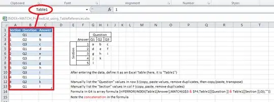
After entering your data, convert it to a table ("Insert", "Table").
List your "Questions" in a row; list your "Rows" down a column. (Note: I took the liberty of renaming your "Row" to "Section" here. I also extended your dataset a bit.)
In cell G4, the formula is
{=IFERROR(INDEX(Table1[Answer],MATCH(G$3 & $F4,Table1[[Question ]] & Table1[Section],0)),"")}
It's an array formula, entered with CTRL+SHIFT+ENTER. Note also the concatenation operator "&" that's used in 2 places. Also note the $ signs, creating absolute references.
Once the array formula has been entered you can drag it across and down.
If you have additional questions or rows to add, just append them to the table object; it will automatically expand to include them. Of course, you'll need to extend your final report's layout to pick up the additions.