Introduction
This article explains how to estimate the coefficients of meromorphic generating functions which have only one dominant singularity.
Theorem
Theorem due to Sedgewick[1].
- If
 is a meromorphic function
- which has only one pole,
 , closest to the origin, with order
- then you can estimate its
 th coefficient with the formula[2]:

Proof
Proof due to Sedgewick[3] and Wilf[4].


 contributes the biggest coefficient. Its th coefficient can be computed as:

 can be computed as:

 as
as  (Proof)
- Therefore, putting it all together:
![{\displaystyle [z^{n}]h(z)\sim {\frac {(-1)^{m}h_{-m}}{a^{m}}}{\binom {n+m-1}{n}}\left({\frac {1}{a}}\right)^{n}\sim {\frac {(-1)^{m}mf(a)}{a^{m}g^{(m)}(a)}}\left({\frac {1}{a}}\right)^{n}n^{m-1}}](../_assets_/eb734a37dd21ce173a46342d1cc64c92/53bfed7d0b8d2ca1052119d9bd3c2afcc1e02c64.svg) as .
as .
Asymptotic equality
We will make use of the asymptotic equality
 as
as 
which means

This allows us to use  as an estimate of
  as
as  gets closer to
  .
.
For example, we often present results of the form
 as
as
which means, for large ,  becomes a good estimate of
  .
.
Meromorphic function
The above theorem only applies to a class of generating functions called meromorphic functions. This includes all rational functions (the ratio of two polynomials) such as  and
and  .
.
A meromorphic function is the ratio of two analytic functions. An analytic function is a function whose complex derivative exists[7].
One property of meromorphic functions is that they can be represented as Laurent series expansions, a fact we will use in the proof.
It is possible to estimate the coefficients of functions which are not meromorphic (e.g.  or
or  ). These will be covered in future chapters.
Laurent series
When we want a series expansion of a function around a singularity  , we cannot use the Taylor series expansion. Instead, we use the Laurent series expansion[8]:

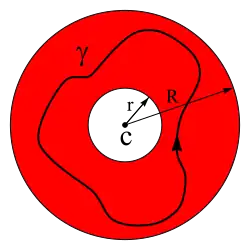
Where  and
and  is a contour in the annular region in which is analytic, illustrated below.
Pole
A pole is a type of singularity.
A singularity of  is a value of for which
  [9]
[9]
If  and
and  is defined then is called a pole of of order [10].
We will make use of this fact when we calculate .
For example,  has the singularity
  because
  and is a pole of order 2 because
  .
.
Closest to the origin
We are treating as a complex function where the input is a complex number.
A complex number has two parts, a real part (Re) and an imaginary part (Im). Therefore, if we want to represent a complex number we do so in a two-dimensional graph.
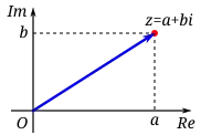
If we want to compare the "size" of two complex numbers, we compare how far they are away from the origin in the two-dimensional plane (i.e. the length of the blue arrow in the above image). This is called the modulus, denoted  .
.
Principle part
Proof due to Wilf[11].
The principle part of a Laurent series expansion are the terms with a negative exponent, i.e.
We will denote the principle part of at by  .
.
If is the pole closest to the origin then the radius of convergence  and as a consequence of the Cauchy-Hadamard theorem[12]:
![{\displaystyle [z^{n}]h(z)\leq \left({\frac {1}{|a|}}+\epsilon \right)^{n}}](../_assets_/eb734a37dd21ce173a46342d1cc64c92/06646f93107497e2e616810991ce75cde35a8f5b.svg) (for some
(for some  and for sufficiently large )
 no longer has a pole at because
  .
.
If the second closest pole to the origin of is  then is the largest pole of and, by the above theorem, the coefficients of
  (for sufficiently large ).
Therefore, the coefficients of are at most different from the coefficient of by  (for sufficiently large ).
Note that if is the only pole, the difference is at most  (for sufficiently large ).
If  then as gets large
  will be much smaller than
  and, therefore, is a good enough approximation of .
However, if  then the behaviour of the coefficients is more complicated.
Biggest coefficient
Compare:
![{\displaystyle [z^{n}]{\frac {h_{-m}}{(z-a)^{m}}}={\frac {h_{-m}}{a^{m}}}{\binom {n+m-1}{n}}\left({\frac {1}{a}}\right)^{n}\sim {\frac {h_{-m}}{a^{m}}}\left({\frac {1}{a}}\right)^{n}n^{m-1}}](../_assets_/eb734a37dd21ce173a46342d1cc64c92/e2c7adb39ee6f29cbd37140cc2381dbc14570ac9.svg) [13]
[13]
with:
![{\displaystyle [z^{n}]{\frac {h_{-(m-1)}}{(z-a)^{m-1}}}={\frac {h_{-(m-1)}}{a^{m-1}}}{\binom {n+m-2}{n}}\left({\frac {1}{a}}\right)^{n}\sim {\frac {h_{-(m-1)}}{a^{m-1}}}\left({\frac {1}{a}}\right)^{n}n^{m-2}}](../_assets_/eb734a37dd21ce173a46342d1cc64c92/e58c1f3b4bec7a572c76af2fac0b04acb39167b7.svg)
The th coefficient of the former is only different to the latter by  .
.
Computation of coefficient of first term
 by factoring out
  .
.
 by the binomial theorem for negative exponents[14].
Computation of h_-m
 .
.
Therefore,  .
.
To compute  , because the numerator and denominator are both
  at , we need to use L'Hôpital's rule[15]:

Indeed, if is a root of order  of and
  , it is also a root of
  and
and  and therefore
  is also indeterminate. Therefore, we need to apply L'Hôpital's rule times:

Proof of binomial asymptotics
 as .
as .
Notes
- ↑ Sedgewick, pp. 59.
- ↑ Sedgewick, (errata), pp. 8.
- ↑ Sedgewick, pp. 59-60.
- ↑ Wilf 2006, pp. 185-186.
- ↑ See Stroud 2003, pp. 919-923, Lang 1999, pp. 161-163, Orloff, pp. 10-13, w:Laurent_series, v:Complex_Analysis_in_plain_view#Laurent_Series_and_the_z-Transform_Example_Note.
- ↑ Wilf 2006, pp. 185-186.
- ↑ Flajolet and Sedgewick 2009, pp. 231.
- ↑ Stroud 2003, pp. 919-920.
- ↑ This is a bit of an over-simplification. For further information, see Stroud 2003, pp. 863-867, 915 and w:Mathematical_singularity.
- ↑ Stroud 2003, pp. 915.
- ↑ Wilf 2006, pp. 52, 185-186.
- ↑ Wilf 2006, pp. 50-52.
- ↑ See #Computation of coefficient of first term and #Proof of binomial asymptotics.
- ↑ Biggs 2002, pp. 364-366.
- ↑ Stroud 2001, pp. 792, v:Calculus/Limits#L'Hôpital's_Rule, w:L'Hôpital's_rule.
References
- Biggs, Norman L. (2002). Discrete Mathematics (2nd ed.). Oxford University Press.
- Flajolet, Philippe; Sedgewick, Robert (2009). Analytic Combinatorics (PDF). Cambridge University Press.
- Lang, Serge (1999). Complex Analysis (4th ed.). Springer Science+Business Media, LLC.
- Orloff, Jeremy. "Topic 7 Notes: Taylor and Laurent series" (PDF). Retrieved 3 October 2022.
- Sedgewick, Robert. "4. Complex Analysis, Rational and Meromorphic Asymptotics" (PDF). Retrieved 16 September 2022.
- Sedgewick, Robert. "4. Complex Analysis, Rational and Meromorphic Asymptotics (Errata)" (PDF). Retrieved 16 September 2022.
- Stroud, K. A. (2003). Advanced Engineering Mathematics (4th ed.). Palgrave Macmillan.
- Stroud, K. A. (2001). Engineering Mathematics (5th ed.). Palgrave Macmillan.
- Wilf, Herbert S. (2006). Generatingfunctionology (PDF) (3rd ed.). A K Peters, Ltd.