Statistics/Distributions/Exponential

Exponential

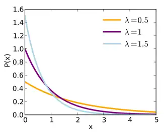
Probability density function
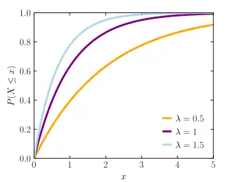
Cumulative distribution function
Parameters	λ > 0 rate, or inverse scale
Support	x ∈ [0, ∞)
PDF	λ e−λx
CDF	1 − e−λx
Mean	λ−1
Median	λ−1 ln 2
Mode	0
Variance	λ−2
Skewness	2
Ex. kurtosis	6
Entropy	1 − ln(λ)
MGF	${\displaystyle \left(1-{\frac {t}{\lambda }}\right)^{-1}\,}$
CF	${\displaystyle \left(1-{\frac {it}{\lambda }}\right)^{-1}\,}$

Exponential distribution refers to a statistical distribution used to model the time between independent events that happen at a constant average rate λ. Some examples of this distribution are:

• The distance between one car passing by after the previous one.
• The rate at which radioactive particles decay.

For the stochastic variable X, probability distribution function of it is:

${\displaystyle f_{x}(x)={\begin{cases}\lambda e^{-\lambda x},&{\mbox{if }}x\geq 0\\0,&{\mbox{if }}x<0\end{cases}}}$

and the cumulative distribution function is:

${\displaystyle F_{x}(x)={\begin{cases}0,&{\mbox{if }}x<0\\{1-e^{-\lambda x}},&{\mbox{if }}x\geq 0\end{cases}}}$

Exponential distribution is denoted as ${\displaystyle X\in {\mbox{Exp(m)}}}$, where m is the average number of events within a given time period. So if m=3 per minute, i.e. there are three events per minute, then λ=1/3, i.e. one event is expected on average to take place every 20 seconds.

We derive the mean as follows.

${\displaystyle \operatorname {E} [X]=\int _{-\infty }^{\infty }x\cdot f(x)dx}$

${\displaystyle \operatorname {E} [X]=\int _{0}^{\infty }x\lambda e^{-\lambda x}dx}$

${\displaystyle \operatorname {E} [X]=\int _{0}^{\infty }(-x)(-\lambda e^{-\lambda x})dx}$

We will use integration by parts with u=−x and v=e^−λx. We see that du=-1 and dv=−λe^−λx.

${\displaystyle \operatorname {E} [X]=\left[-x\cdot e^{-\lambda x}\right]_{0}^{\infty }-\int _{0}^{\infty }(e^{-\lambda x})(-1)dx}$

${\displaystyle \operatorname {E} [X]=[0-0]+\left[{-1 \over \lambda }(e^{-\lambda x})\right]_{0}^{\infty }}$

${\displaystyle \operatorname {E} [X]=\left[0-{-1 \over \lambda }\right]}$

${\displaystyle \operatorname {E} [X]={1 \over \lambda }}$

We use the following formula for the variance.

${\displaystyle \operatorname {Var} (X)=\operatorname {E} [X^{2}]-(\operatorname {E} [X])^{2}}$

${\displaystyle \operatorname {Var} (X)=\int _{-\infty }^{\infty }x^{2}\cdot f(x)dx-\left({2}\right)^{2}}$

${\displaystyle \operatorname {Var} (X)=\int _{0}^{\infty }x^{2}e^{-2x}dx-{2}}$

We'll use integration by parts with ${\displaystyle u=-x^{2}}$ and ${\displaystyle v=e^{-2x}}$. From this we have ${\displaystyle du=-2x}$ and ${\displaystyle v=-2e^{-2x}}$.

${\displaystyle \operatorname {Var} (X)=\left\{\left[-x^{2}\cdot e^{-\lambda x}\right]_{0}^{\infty }-\int _{0}^{\infty }(e^{-\lambda x})(-2x)dx\right\}-{1 \over \lambda ^{2}}}$

${\displaystyle \operatorname {Var} (X)=[0-0]+{2 \over \lambda }\int _{0}^{\infty }x\lambda e^{-\lambda x}dx-{1 \over \lambda ^{2}}}$

We see that the integral is just ${\displaystyle \operatorname {E} [X]}$ which we solved for above.

${\displaystyle \operatorname {Var} (X)={2 \over \lambda }{1 \over \lambda }-{1 \over \lambda ^{2}}}$

${\displaystyle \operatorname {Var} (X)={1 \over \lambda ^{2}}}$

• Interactive Exponential Distribution Web Applet (Java)