Statistics/Distributions/Geometric

Geometric

Probability mass function
Cumulative distribution function
Parameters	${\displaystyle 0<p\leq 1}$ success probability (real)
Support	${\displaystyle k\in \{1,2,3,\dots \}\!}$
PMF	${\displaystyle (1-p)^{k-1}\,p\!}$
CDF	${\displaystyle 1-(1-p)^{k}\!}$
Mean	${\displaystyle {\frac {1}{p}}\!}$
Median	${\displaystyle \left\lceil {\frac {-1}{\log _{2}(1-p)}}\right\rceil \!}$ (not unique if ${\displaystyle -1/\log _{2}(1-p)}$ is an integer)
Mode	${\displaystyle 1}$
Variance	${\displaystyle {\frac {1-p}{p^{2}}}\!}$
Skewness	${\displaystyle {\frac {2-p}{\sqrt {1-p}}}\!}$
Ex. kurtosis	${\displaystyle 6+{\frac {p^{2}}{1-p}}\!}$
Entropy	${\displaystyle {\tfrac {-(1-p)\log _{2}(1-p)-p\log _{2}p}{p}}\!}$
MGF	${\displaystyle {\frac {pe^{t}}{1-(1-p)e^{t}}}\!}$, for ${\displaystyle t<-\ln(1-p)\!}$
CF	${\displaystyle {\frac {pe^{it}}{1-(1-p)\,e^{it}}}\!}$

There are two similar distributions with the name "Geometric Distribution".

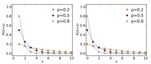
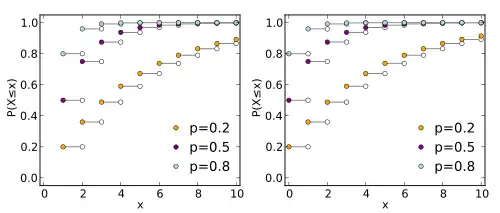
• The probability distribution of the number X of Bernoulli trials needed to get one success, supported on the set { 1, 2, 3, ...}

• The probability distribution of the number Y = X − 1 of failures before the first success, supported on the set { 0, 1, 2, 3, ... }

These two different geometric distributions should not be confused with each other. Often, the name shifted geometric distribution is adopted for the former one. We will use X and Y to refer to distinguish the two.

The shifted Geometric Distribution refers to the probability of the number of times needed to do something until getting a desired result. For example:

• How many times will I throw a coin until it lands on heads?
• How many children will I have until I get a girl?
• How many cards will I draw from a pack until I get a Joker?

Just like the Bernoulli Distribution, the Geometric distribution has one controlling parameter: The probability of success in any independent test.

If a random variable X is distributed with a Geometric Distribution with a parameter p we write its probability mass function as:

${\displaystyle P\left(X=i\right)=p\left(1-p\right)^{i-1}}$

With a Geometric Distribution it is also pretty easy to calculate the probability of a "more than n times" case. The probability of failing to achieve the wanted result is ${\displaystyle \left(1-p\right)^{k}}$.

Example: a student comes home from a party in the forest, in which interesting substances were consumed. The student is trying to find the key to his front door, out of a keychain with 10 different keys. What is the probability of the student succeeding in finding the right key in the 4th attempt?

${\displaystyle P\left(X=4\right)={\frac {1}{10}}\left(1-{\frac {1}{10}}\right)^{4-1}={\frac {1}{10}}\left({\frac {9}{10}}\right)^{3}=0.0729}$

The probability mass function is defined as:

${\displaystyle f(x)=p(1-p)^{x}\,}$ for ${\displaystyle x\in \{0,1,2,\dots \}}$

${\displaystyle \operatorname {E} [X]=\sum _{i}f(x_{i})x_{i}=\sum _{0}^{\infty }p(1-p)^{x}x}$

Let q=1-p

${\displaystyle \operatorname {E} [X]=\sum _{0}^{\infty }(1-q)q^{x}x}$

${\displaystyle \operatorname {E} [X]=\sum _{0}^{\infty }(1-q)qq^{x-1}x}$

${\displaystyle \operatorname {E} [X]=(1-q)q\sum _{0}^{\infty }q^{x-1}x}$

${\displaystyle \operatorname {E} [X]=(1-q)q\sum _{0}^{\infty }{\frac {d}{dq}}q^{x}}$

We can now interchange the derivative and the sum.

${\displaystyle \operatorname {E} [X]=(1-q)q{\frac {d}{dq}}\sum _{0}^{\infty }q^{x}}$

${\displaystyle \operatorname {E} [X]=(1-q)q{\frac {d}{dq}}{1 \over 1-q}}$

${\displaystyle \operatorname {E} [X]=(1-q)q{1 \over (1-q)^{2}}}$

${\displaystyle \operatorname {E} [X]=q{1 \over (1-q)}}$

${\displaystyle \operatorname {E} [X]={(1-p) \over p}}$

We derive the variance using the following formula:

${\displaystyle \operatorname {Var} [X]=\operatorname {E} [X^{2}]-(\operatorname {E} [X])^{2}}$

We have already calculated E[X] above, so now we will calculate E[X²] and then return to this variance formula:

${\displaystyle \operatorname {E} [X^{2}]=\sum _{i}f(x_{i})\cdot x^{2}}$

${\displaystyle \operatorname {E} [X^{2}]=\sum _{0}^{\infty }p(1-p)^{x}x^{2}}$

Let q=1-p

${\displaystyle \operatorname {E} [X^{2}]=\sum _{0}^{\infty }(1-q)q^{x}x^{2}}$

We now manipulate x² so that we get forms that are easy to handle by the technique used when deriving the mean.

${\displaystyle \operatorname {E} [X^{2}]=(1-q)\sum _{0}^{\infty }q^{x}[(x^{2}-x)+x]}$

${\displaystyle \operatorname {E} [X^{2}]=(1-q)\left[\sum _{0}^{\infty }q^{x}(x^{2}-x)+\sum _{0}^{\infty }q^{x}x\right]}$

${\displaystyle \operatorname {E} [X^{2}]=(1-q)\left[q^{2}\sum _{0}^{\infty }q^{x-2}x(x-1)+q\sum _{0}^{\infty }q^{x-1}x\right]}$

${\displaystyle \operatorname {E} [X^{2}]=(1-q)q\left[q\sum _{0}^{\infty }{\frac {d^{2}}{(dq)^{2}}}q^{x}+\sum _{0}^{\infty }{\frac {d}{dq}}q^{x}\right]}$

${\displaystyle \operatorname {E} [X^{2}]=(1-q)q\left[q{\frac {d^{2}}{(dq)^{2}}}\sum _{0}^{\infty }q^{x}+{\frac {d}{dq}}\sum _{0}^{\infty }q^{x}\right]}$

${\displaystyle \operatorname {E} [X^{2}]=(1-q)q\left[q{\frac {d^{2}}{(dq)^{2}}}{1 \over 1-q}+{\frac {d}{dq}}{1 \over 1-q}\right]}$

${\displaystyle \operatorname {E} [X^{2}]=(1-q)q\left[q{2 \over (1-q)^{3}}+{1 \over (1-q)^{2}}\right]}$

${\displaystyle \operatorname {E} [X^{2}]={2q^{2} \over (1-q)^{2}}+{q \over (1-q)}}$

${\displaystyle \operatorname {E} [X^{2}]={2q^{2}+q(1-q) \over (1-q)^{2}}}$

${\displaystyle \operatorname {E} [X^{2}]={q(q+1) \over (1-q)^{2}}}$

${\displaystyle \operatorname {E} [X^{2}]={(1-p)(2-p) \over p^{2}}}$

We then return to the variance formula

${\displaystyle \operatorname {Var} [X]=\left[{(1-p)(2-p) \over p^{2}}\right]-\left({1-p \over p}\right)^{2}}$

${\displaystyle \operatorname {Var} [X]={(1-p) \over p^{2}}}$

• Interactive Geometric Distribution Web Applet (Java)