Python: normalised cumulative distribution function from array of probability density function

Question

For a continuous variable x and its probability density function p(x), I have a numpy array of x values x and a numpy array of corresponding p(x) values p. p(x) is not normalised though, i.e. in a plot of p(x) against x, the area under the graph is not 1. I want to calculate a corresponding array for values of the cumulative distribution function cdf. This is how I'm currently doing it, using the Trapezoidal rule to approximate an integral:

p_norm = p/np.trapz(p,x)
cdf = np.array([np.trapz(p_norm[:n],x[:n]) for n in range(len(p_norm))])

The results aren't entirely accurate; the final value of cdf is close to 1 but not exactly 1.

Is there any more accurate and simple way of normalising p and finding cdf? I thought there might be specific functions for this in some module; perhaps a statistics-oriented module with functions for related parameters (variance, confindence intervals etc) as well?

You can normalise `p` with `p / np.sum(p)` and then the CDF is `np.cumsum(p)`. — Reti43, Mar 11 '21 at 15:55
@Reti43 I think that works when x is a discrete variable, but not when its a continuous variable. — o c, Mar 11 '21 at 16:09
Do you have an expression for p, or do you have a lot of samples instead? — Reti43, Mar 11 '21 at 21:14
@Reti43 No, I don't have an expression for p(x), just an array of x values and an array of the corresponding p(x) values. The number of values in the arrays is typically large though. — o c, Mar 11 '21 at 21:40
Try using some of the other methods I mentioned in the [answer](https://stackoverflow.com/a/66593155/8474894). Also take a look at [`scipy.integrate.cumulative_trapezoid`](https://docs.scipy.org/doc/scipy/reference/generated/scipy.integrate.cumulative_trapezoid.html) for evaluating the `cdf`. — CypherX, Mar 12 '21 at 02:41
A lot of samples != continuous. Your best bet is to integrate the area under your sampled curve and normalize with that. Your normalization factor will be only for the sampled area you have captured and will not be equal to the continuous one (if it has an expression). But assuming what you've left out from the tails is very small, it should be close enough. — Reti43, Mar 12 '21 at 13:59

CypherX · Answer 1 · 2021-03-12T02:47:22.737

Methods of Integration for Discrete Data-points

The variable x is only continuous if you have a continuous functional form for it. If you have a few discrete values (which it will be if you were to make a numpy array of discrete values), then the array is no longer continuous as it can not resolve points in between two successive discrete values of x.

So, assuming that you, in effect have an array of discrete data-points for both x and p, here are my suggestions.

Get Acquainted With a Few Methods of Numerical Integration First

Newton-Cotes Formulas | Code: scipy.integrate.newton_cotes

This is a generic rule comprising of integration using n-points. If we denote the n-point formula as: newton-cotes(n), then
- Trapezoidal Rule: n = 2 | Code: scipy.integrate.trapezoid
- Simpson's Rule: n = 3 | Code: scipy.integrate.simpson
- Simpson's 3/8 Rule: n = 4
- Boole's Rule: n = 5 | Code: See this for an idea.
Weddle's Rule
Hardy's Rule

1. Integrate using `scipy.integrate`

You can use any of the methods listed under "Methods for Integrating Functions given fixed samples".

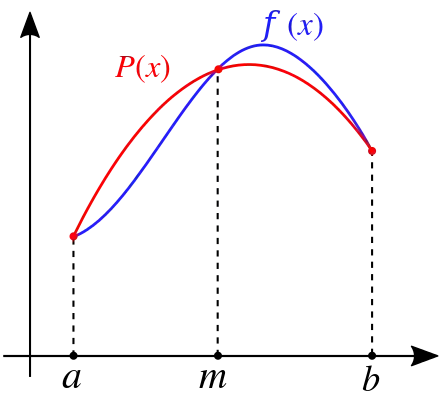
INSIGHT What is important here is: in trapezoidal rule you interpolate the space between the successive two points using a straight line. If you could use a higher order polynomial (order ~ 2, 3, 4, etc.) then that could give you a better result for integration. Simpson's rule uses 2nd-order polynomial Simpson's Rule - Wolfram MathWorld.


Simpson's Rule: Integrating area under a curve using quadratic polynomials	An animation showing how Simpson's Rule is applied for integration

^{Source: Wikipedia}

Methods for Integrating Functions given fixed samples

   trapezoid            -- "Use trapezoidal rule to compute integral."
   cumulative_trapezoid -- "Use trapezoidal rule to cumulatively compute integral."
   simps                -- "Use Simpson's rule to compute integral from samples."
   romb                 -- "Use Romberg Integration to compute integral from
                           (2**k + 1) evenly-spaced samples."

Also see this for a quick example: Calculating the area under a curve given a set of coordinates, without knowing the function.

2. Area Under the Curve (AUC) using `sklearn.metrics.auc`

Integration is in essence the area under a curve (AUC). Scikit-learn library provides an easy alternative to calculating AUC. In practice this also uses the trapezoidal rule and so, I do not see any reason why this should be any/much different from what you already have using numpy.trapz.

Docs - sklearn.metrics.auc
Example: auc = sklearn.metrics.auc(x, y)

3. Consider using Other Methods

3.1. Romberg Integration

scipy.integrate.romb(y, dx=1.0, axis=- 1, show=False)

Docs: scipy.integrate.romb
What is Romberg's Method?
- Wikipedia
- Math behind Romberg Integration: PDF
- YouTube Video: Numerical Integration - Romberg Integration - example

References

You go in detail discussing various integration methods and you miss out the key point that it should be normalized. Easy fix, but it really needs to be included. — Reti43, Mar 12 '21 at 14:01
@Reti43 Normalization is a part of defacto steps (anyone who understands probabilities would normalize either before or after integration -- both works; but I would prefer normalizing before). The OP asked for other methods -- so I shared those to let compare apples to apples. When you integrate something using various methods, the input must be kept the same for comparison. Besides, you had told the OP to normalize. Didn't see any point in mentioning it once again. — CypherX, Mar 12 '21 at 15:41