How to plot points across time when the years are different columns?

Question

So I'm trying to plot points across time when the years are different columns but I've failed so far because of the figure margins too large error. I emailed my TA and he said to look this up on google because it looks like I'm trying to plot the whole dataset instead of different variables. I'm trying to plot the points for this country called specifically Argentina in the year 1960 to 1974. Hope you guys can help :)

I'm using this csv file from this website: https://data.worldbank.org/indicator/NY.GDP.PCAP.KD

I've tried to use:

library(dplyr)

Argentina <- gdp %>% 
  filter(country ==  "Argentina")

plot(Argentina)

Welcome to Stack Overflow. It will be easier for people to give you useful help if you can edit your question to include some sample data as code. For instance, if you run `dput(head(Argentina))`, R will produce code that you can include in your question so that we can be working from exactly the same form of data (the first 6 rows, in this case) that you have. — Jon Spring, Jul 08 '23 at 20:17
I suspect the solution could involve using `pivot_longer` (from `tidyr`, included with `tidyverse`) to reshape your data so that the multiple columns you want are combined into a pair of columns, one denoting the year and one with the values. Hard to know for sure without example data. — Jon Spring, Jul 08 '23 at 20:21
See: https://stackoverflow.com/questions/2185252/reshaping-data-frame-from-wide-to-long-format — Jon Spring, Jul 08 '23 at 20:33
Actually, `plot(Argentina)` is not data, it's a plotting instruction. What @JonSpring is saying is that if you include data you wont be forcing us to download a file from that page. Jon did read the post correctly. — Rui Barradas, Jul 08 '23 at 21:06

Rui Barradas · Answer 1 · 2023-07-08T22:31:59.633

1

This type of problems generally has to do with reshaping the data. The format should be the long format and the data is in wide format. See this post on how to reshape the data from wide to long format.
I will use pivot_longer from package tidyr after some data prep.

csv <- "API_NY.GDP.PCAP.KD_DS2_en_csv_v2_5607189.csv"
gdp <- read.csv(csv, skip = 4L, check.names = FALSE)
gdp <- gdp[-grep("Indicator", names(gdp))]
gdp <- gdp[-ncol(gdp)]


suppressPackageStartupMessages({
  library(dplyr)
  library(tidyr)
})

Argentina <- gdp %>%
  filter(country == "Argentina") %>%
  pivot_longer(-country, names_to = "Year", values_to = "GDP") %>% 
  mutate(Year = as.integer(Year)) %>%
  select(Year, GDP)

^{Created on 2023-07-08 with reprex v2.0.2}

Base R plot

This is a one-line plot.

plot(Argentina)

^{Created on 2023-07-08 with reprex v2.0.2}

Package `ggplot2`

library(ggplot2)

ggplot(Argentina, aes(Year, GDP)) +
  # geom_line() +
  geom_point() +
  ggtitle("Argentina") +
  ylab("GDP per capita (constant 2015 US$)") +
  theme_bw()

^{Created on 2023-07-08 with reprex v2.0.2}

edited Jul 08 '23 at 22:31

answered Jul 08 '23 at 21:03

Rui Barradas

70,273
8
34
66

Hi, so I've just tried to copy and paste what you wrote into r and it's giving me the error code of "Error in `filter()`: ℹ In argument: ``Country Name` == "Argentina"`. Caused by error: ! object 'Country Name' not found" ? – Cassie Tran Jul 08 '23 at 21:45
@CassieTran Try the name in your post, `country`. The data file has the name written like in my answer, that's all. – Rui Barradas Jul 08 '23 at 21:48
Hi, I've also tried to copy and paste "ggplot(Argentina, aes(1960, 7410), (1961, 7690)) + # geom_line() + geom_point() + ggtitle("Argentina") + ylab("GDP per capita (constant 2015 US$)") + theme_bw()" but it's giving me the error code of "Error: unexpected ',' in "ggplot(Argentina, aes(1960, 7410), (1961,"". Hope you can help! :) – Cassie Tran Jul 08 '23 at 21:49
@CassieTran This is meaningless: `aes(1960, 7410), (1961, 7690))`, it's not R code. Run `str(Argentina)` to see the name of the country column and use that name in the ggplot `aes`. – Rui Barradas Jul 08 '23 at 21:52
Hi Rui, I've just tried to run str(Argentina) and also I've rewritten the code as ggplot(Argentina, Argentina(Year, GDP)) + like you said but it's still giving me the error message of "Error in Argentina(Year, GDP) : could not find function "Argentina""? – Cassie Tran Jul 08 '23 at 22:01
@CassieTran It's `ggplot(Argentina, aes(Year, GDP))` – Rui Barradas Jul 08 '23 at 22:10
@CassieTran And I made a mistake in my earlier comment, in `filter('Country Name' == "Argentina")` use the country column name returned by the `str(gdp)` instruction. – Rui Barradas Jul 08 '23 at 22:11
Hi Rui, I'm not quite sure I understand what you mean? Can you please type out the full code for me please? Because when I've typed in "str(gdp) ggplot(Argentina, aes(Year, gdp)) +" it's giving me the error code of "Error in geom_point() : ℹ Error occurred in the 1st layer. Caused by error: ! object 'Year' not found" And thank you so much! – Cassie Tran Jul 08 '23 at 22:15
@CassieTran 1) run `str(gdp)`. What is the country column name? – Rui Barradas Jul 08 '23 at 22:19
Hi @RuiBarradas https://imgur.com/a/ugd1DtW, this is what shows up when I run str(gdp), I'm not sure what you mean by country column name? – Cassie Tran Jul 08 '23 at 22:23
@CassieTran The filter instruction should be `filter(country == "Argentina") %>%`. The rest of the code should run fine, give it a try and if not post a picture of the exact code you ran and the error message like you did, please. – Rui Barradas Jul 08 '23 at 22:26
And also, when I've tried the first answer that you gave me in this chat by changing "Country Name" to just "country" it's giving me the error message of Error in `filter()`: ℹ In argument: `country == "Argentina"`. Caused by error: ! object 'country' not found" as well? – Cassie Tran Jul 08 '23 at 22:27
https://imgur.com/a/scmeB3Q https://imgur.com/a/wmis6Mi these are the codes that I have in r so far and also the second image is the error that I've been receiving? – Cassie Tran Jul 08 '23 at 22:31
@CassieTran In the first picture you have posted there is a column named `country`. Is the `filter` being applied to the same data.frame? Also, read the data file with `check.names = FALSE` to get rid of the `X` before the year. – Rui Barradas Jul 08 '23 at 22:35
Hi no, there is a not a name for the country called Argentina. If you can take a look at these two images for me, I don't see any data that matches up with 7140 to begin with which is Argentina's GDP for 1960. https://imgur.com/a/jEfEiif https://imgur.com/a/T9SqDxZ And yes I've just reran the codes with check.names = + FALSE like you mentioned – Cassie Tran Jul 08 '23 at 22:57
@CassieTran In the first picture it says `211 Obs. of 63 variables`. The first of those variables is `country`. If you reran the code to read the file with `check.names = FALSE`, can you post the new `str(gdp)`? The problem here doesn't seem to be with the plot, it is a problem with the data. – Rui Barradas Jul 08 '23 at 23:02
Hi @RuiBarradas, the new str(gdp) is the pictures that I just posted sir. – Cassie Tran Jul 08 '23 at 23:04
Actually I've just found the country code name, it's ARG. And now I've substituted Argentina for ARG it's giving me the error message of "ARG not found" I've also included my codes in these photos and the error message that I've received https://imgur.com/a/xdKHzLE https://imgur.com/a/NDDMiSe – Cassie Tran Jul 08 '23 at 23:15

jay.sf · Accepted Answer · 2023-07-09T08:56:53.600

0

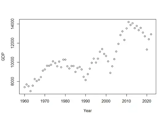
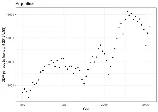
There is actually no need to mess with the data. R has a built-in plotting function for matrices, matplot.

We can already get a base plot using just:

matplot(t(gdp.ARG), type='l')

Or, for the Latin American countries:

matplot(t(gdp.LAT), type='l')

We can fine-tune this:

labs <- as.integer(sub('X', '', names(gdp.ARG)))
y10 <- labs %% 10 == 0

matplot(t(gdp.LAT), type='l', xaxt='n', yaxt='n', main='Latin America',
        xlab='Year', ylab='GDP p. cap.',  ylim=c(0, max(gdp.LAT, na.rm=TRUE)),
        panel.first={abline(v=seq_along(labs)[y10], lty=3, col='grey80');
          abline(h=seq.int(0, max(gdp.LAT, na.rm=TRUE), 5e3), lty=3, col='grey80')})
axis(2, axTicks(2), labels=paste(axTicks(2)/1e3, 'K'), tck=-.01, las=2)
axis(1, seq_along(gdp.LAT), labels=FALSE, tck=-.01)
axis(1, seq_along(gdp.LAT)[y10], labels=FALSE)
mtext(labs[y10], side=1, line=1, at=seq_along(labs)[y10])
legend('topleft', col=1:6, lty=1:5,
       legend=rownames(gdp.LAT)[-nrow(gdp.LAT)], ncol=4, cex=.8)  ## `col`ors and `lty`s as `matplot`, may not exceed 6*5=30 units, else use different strategy

Note, that Venezuela is missing in the data.

Data:

tmp <- tempfile()  ## open a tempfile connection
download.file(paste0('https://api.worldbank.org/v2/en/indicator/',
                     'NY.GDP.PCAP.KD?downloadformat=csv'), tmp)  ## download file from World Bank
dat <- read.csv(unz(tmp, 'API_NY.GDP.PCAP.KD_DS2_en_csv_v2_5607189.csv'), 
                skip=4)  ## read it
unlink(tmp)  ## close temp connection

head(dat)  ## look into `head` instead of using the silly `View`er

rownames(dat) <- dat$Country.Code  ## suitable, since we have distinct country codes

gdp.ARG <- dat[dat$Country.Code == 'ARG', c(5:67)]  ## extract ARG
gdp.LAT <- dat[dat$Country.Code %in% c("ARG", "BOL", "BRA", "CHL", "COL", "ECU",
                                       "GUY", "PER", "PRY", "SUR", "URY", 
                                       "VEN"), c(5:67)]  ## extract Latin America

edited Jul 09 '23 at 08:56

answered Jul 09 '23 at 08:02

jay.sf

60,139
8
53
110

Hi @jay.sf , so I just tried to copy and paste matplot(t(gdp.ARG), type='l') into r and it's giving me the error code of "Error: object 'gdp.ARG' not found" – Cassie Tran Jul 09 '23 at 08:18
@CassieTran Did you execute the code in section _Data_? – jay.sf Jul 09 '23 at 08:22
Hi Jay! So I just executed the code in the section Data and it worked beautifully! Thank you so much for your help! Also, I'm just wondering if I want to one for China what would it look like? Would it look like this? gdp.CHN <- dat[dat$Country.Code == 'CHN', c(5:67)] – Cassie Tran Jul 09 '23 at 08:42
@CassieTran Yes, exactly, impressed you learned it so quickly :) – jay.sf Jul 09 '23 at 08:46
@CassieTran For convenience, you can also do `matplot(t(subset(dat, Country.Code == 'CHN')), type='l')`, where `subset(dat, Country.Code == 'CHN')` is equivalent to `dat[dat$Country.Code == 'CHN', ]`. – jay.sf Jul 09 '23 at 08:49
Hi @jay.sf, can you also add in the comments here on how I can fine tune the plot for China then? I’m a bit confused on what to change by just looking at the example you gave for Latin America because I only want the fine tuned version of just 1 country and not of a whole bunch of different ones? – Cassie Tran Jul 09 '23 at 08:50
@CassieTran You can use the same code, just use gdp.CHN (also in `ylim`) and you need `abline(h=seq.int(0, max(gdp.CHN, na.rm=TRUE), by=2e3)`, but you would have figured that out. And the legend would be obsolete I guess. – jay.sf Jul 09 '23 at 09:00
Hi @jay.sf , so I just typed in what you told me to type in and it's giving me the error code of "labs not found". I've included a photo of what my r data codes look like if that helps ? https://imgur.com/a/jQ7JGdE – Cassie Tran Jul 09 '23 at 09:11
@CassieTran `labs` is created directly after _"We can fine-tune this:"_. I forgot to include it before my edit. – jay.sf Jul 09 '23 at 09:14
Amazing !! This worked wonderfully !! Also if you have some time can you also look at the new question that I just posted? Thanks ! Hope it's not too much to ask – Cassie Tran Jul 09 '23 at 09:31

How to plot points across time when the years are different columns?

2 Answers2

Base R plot

Package `ggplot2`

Linked

How to plot points across time when the years are different columns?

2 Answers2

Base R plot

Package ggplot2

Linked

Package `ggplot2`