-1

I am using SharePoint to collect data through its survey feature. However, I want to make the output data more manageable. As such, I want to take the multiple columns and consolidate them into a few.

Currently, it looks like this:

Name 1  Address 1  Age 1 Name 2 Address 2 Age 2 Name 3 Address 3 Age 3 Date

John    My Home   50 Mary Your Home 40 James Our Home 70 01/31/1991 

I want it to look like this:

**Name Address Age Date** 

John My Home 50  01/31/1991 

Mary Your Home 40 01/31/1991

James Our Home 70 01/31/1991

The survey is continuously updates, so, ideally a macro/vba that extract the data from one sheet and produces it this way, would be better.

Also, a word of caution is that sometimes the cells in either column may be empty. So I want to make sure the formula just doesn't stop because it sees a blank cell, but rather copy from top to bottom from one column to the other.

Last but not least, there is other data in the cells, with other steps I would probably add to the macro, but this is the bulk of the steps I couldn't figure.

Thanks in advance for your help !

Similar Query (it seems) : Excel 2010 Move data from multiple columns/rows to single row

Joel
  • 1

1 Answers1

0

There's a simple way to do this without VBA, just using cell references. It looks like your "source" example uses columns A:J and I'll assume there are column headings, so the data starts in row 2. I'll assume your output sheet also has column headingss and the results start in row 2, and use columns A:D. The formulas, below, are based on this layout, so you may need to adjust for a different layout or just put the data in those locations. So here is the source data:

Source

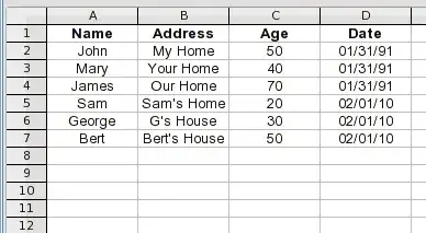
The result looks like this:

Result

The whole thing uses "11/2" formulas. Since the date is referenced from the same place for three rows, it's a slightly modified version of the main formula. The main formula is:

=INDIRECT("sheet1!r"&CEILING((ROW()-1)/3,1, )+1&"c"&COLUMN()+MOD((ROW()+1)/3,1)*9,0)

You can enter it in A2 and copy it to columns B and C, and copy it down to pre-populate as many rows as you need. When you need more, just pre-populate an arbitrary number of additional rows.

It uses the INDIRECT function to create cell references from calculated values. I'm using R1C1 style addresses because they lend themselves to these kinds of calculations. The row calculation produces a reference to the same source row for three output rows. The column calculation moves over three source columns for each successive result row.

The date column just fixes the column reference to column 10 of the source:

=INDIRECT("sheet1!r"&CEILING((ROW()-1)/3,1, )+1&"c10",0)

This produces an output of 0 for empty source cells. The easiest way to hide that is to set the page view to not display zero values. I did that here. The formula is pre-populated in the rows beyond Bert. It will also hide individual empty cells.

fixer1234
  • 28,064