1

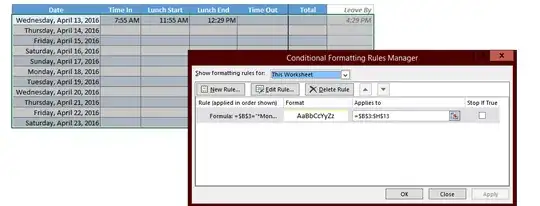
I know this has been asked before, but I must be missing something. I want to put a border above all rows that contain "Monday".

enter image description here

The formula is =$B$3="*Monday*"

I thought it might be because the value of the cell is actually "4/18/2016" but I manually changed it to "Monday" and the rule still didn't fire. What am I doing wrong?
THE JOATMON
  • 1,975
  • 14
  • 54
  • 90

3 Answers3

2

Having the formula pointing on $B$3 will always be true or false, if $B$3 is Monday or not. You need to make the row a relativ reference, ie the formula should be something like =IF($B3="Monday";TRUE;FALSE).

The omitted $ in front of the row will make this formula look into the first column in every row, thus making a border around all mondays.

In order to improve the formula and assuming that you have a date value in your date column, I would recommend to use the function WEEKDAY() and to check for the numeric value of the weekday (see Microsoft Help).

Vince42
  • 311
  • 1
  • 8
1

Use the WEEKDAY() function.

Syntax: WEEKDAY(serial_number,[return_type])

Use this formula in your conditional format, assuming column A contains your dates.

=WEEKDAY(A1,2)=1

With the return type of 2, it starts the week with Monday being the 1st day. So the formula will identify the weekdays that are equal to 1 then format them with your rule.

CharlieRB
  • 23,021
  • 6
  • 60
  • 107
1

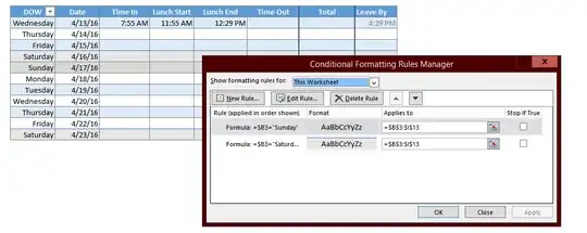
The problem was two-fold. I fixed the formula to be =$B3="Monday". I also had to create an additional column with the formula of =TEXT(C3,"dddd") so that the value was actually "Monday". As it was before, the content of the cell being "2016/4/18", it was only displaying Monday due to the cell format. This never triggered the condition.

Here is the result with Monday replaced by Saturday and Sunday.

enter image description here

THE JOATMON
  • 1,975
  • 14
  • 54
  • 90