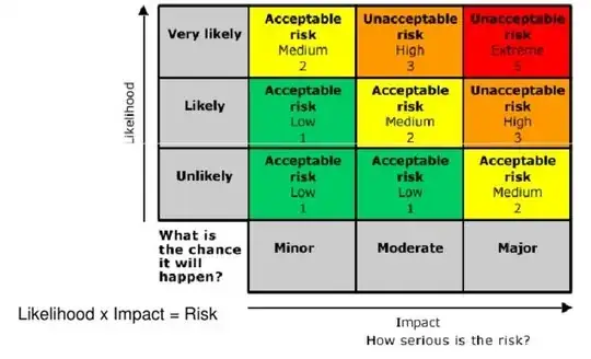
Personally, I'd create the risk chart as a table and then use index match pairs to find the row and column to locate the result you are seeking.
=index(RISK_TABLE_RANGE,MATCH(Likelihood_Cell,Likelihood_Range_RISKTABLE,0),
 MATCH(Risk_Cell,Impact_Range_RISKTABLE,0))
Essentially, you have the entire RISK_TABLE as one range and two additional ranges Likelihood_Range and Impact_Range which are the header/index for your risk table. You match on the two ranges and you get the cell coordinates for the RISK Level which appears in the square.
Think of it as a game of battleship where you ask "what row does very unlikely appear" and then "what column does major appear"