0

I have a list of data from 2015-2016 and want to keep the two years together based on a common data point. I would also like to exclude anything that does not have both years on file because I only care about the year to year change, so single values are just clutter.

So my table looks something like this. I want to take out the "oranges" line. Thanks!

edit: and by "apples" "pears" etc., I mean, unique reference numbers--these being the data point that I would like to connect the years to.

2015    apples  4   $0.79
2016    apples  2   $0.83
2016    oranges 14  $1.12
2015    pears   22  $0.74
2016    pears   17  $0.79
Jeb
  • 9

3 Answers3

1

You can use a formula that return 2 for the connected items and 1 for non duplicate:

=COUNTIFS($A$1:$A$8,2015,$B$1:$B$8,B1)+COUNTIFS($A$1:$A$8,2016,$B$1:$B$8,B1)

$A$1:$A$8 the year column change it to correspond your Data and keep $
$B$1:$B$8 the fruit column change it to correspond your Data and keep $
B1 the fruit that you want to count
Drag the formula down the column
Sort all the Data by the countifs 2 will be together and 1 together, you can delete the rows with 1

yass
  • 2,574
0

This isn't the MOST elegant solution but it works.

In your example, I would sort by Column A then by Column B so all of your data is in the format above predictably. Then, add these statements:

2015    apples  4   $0.79         $STM2  $STM3
2016    apples  2   $0.83  $STM1  $STM2  $STM3
2016    oranges 14  $1.12  $STM1  $STM2  $STM3
2015    pears   22  $0.74  $STM1  $STM2  $STM3
2016    pears   17  $0.79  $STM1         $STM3

So for line 2 that $STM# are equal to: $STM1 =

=IF(B2=B1,TRUE,FALSE)

$STM2 =

=IF(B2=B3,TRUE,FALSE)

$STM3 =

=IF(E2=F2,TRUE,FALSE)

For all entries where $STM3 = TRUE, delete the line. In my example it looked like this:

2015    apples  4   $0.79          TRUE   FALSE
2016    apples  2   $0.83   TRUE   FALSE  FALSE
2016    oranges 14  $1.12   FALSE  FALSE  TRUE
2015    pears   22  $0.74   FALSE  TRUE   FALSE
2016    pears   17  $0.79   TRUE          FALSE
Will
  • 1,492
  • 1
  • 9
  • 27
0

Based on the linked duplicate:

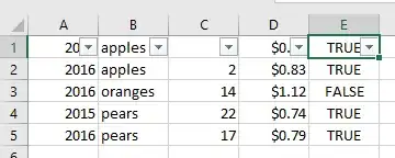
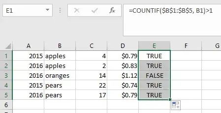
  1. Create a new helper column, using =COUNTIF($B$1:$B$5, B1) at the start of the column, and drag it down to the end of range.

Helper column

  1. Press Ctrl+Shift+L to turn Filtering on.

Filtering on

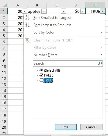
  1. Click on the little down arrow on the helper column, and uncheck TRUE

Filter out TRUE values

  1. It will leave you with only FALSE values. Select all rows with FALSE and delete them.

Note: the topmost row is considered header and thus will always visible regardless of the value.

Only FALSE

  1. Again, click the little down arrow, and check back the TRUE values. Then you can turn off filtering by pressing Ctrl+Shift+L

Taken, and adapted, from: How to remove non-duplicate records in Excel-2010

Vylix
  • 1,935