LibreOffice: count distinct values from column

Question

I have a column with some repeatable values, like color names in a list of a material objects. How could I count a number of each unique value occurrences (e.g. for the 100 rows given there are 5 red, 15 green and 80 black)? I cant use COUNTIF since I don't know all the "colors" that may occure.

In SQL-way I would do something like

SELECT count(`color`), `color` FROM `MyTable` goup by `color`

Answer 1

A spreadsheet cannot do it as easily as with SQL, but here are two solutions.

Method 1 - Pivot Table

Make sure the first row of the column contains a label, for example Color. In the next column, set the label to Count. Enter a count of 1 for all colors.

Color  Count
red    1
green  1
red    1

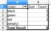
Then, select the two columns and go to Data -> Pivot Table -> Create. Drag Color to Row Fields, and drag Count to Data Fields.

Method 2 - Filter

1. Copy the column data, and paste into column A of a new sheet.
2. Go to Data -> More Filters -> Standard Filter.
3. Change Field Name to - none -. Expand Options and check No duplicates. Press OK.
4. In B1, enter the formula =COUNTIF($Sheet1.G1:G100,"="&A1). Change "G" to the column you used on Sheet 1.
5. Drag the formula down.

Links for getting distinct values are at https://stackoverflow.com/a/38286032/5100564.

Answer 2

Another simple option:

Assumptions:

• Your data is sorted
• For the example below your data is in column A (adjust accordingly).
• For the example below you enter the formula on row 2.

Add a new column with the formula below created on row 2 and copy it to all other rows.

IF(A2 == A1, 0, 1)

Then you get a 1 in that column ever time a value differs from the row above. Then you can just sum the 1 values:

SUM(B2:B?)

Your spreadsheet would look like this:

 1  "A" | "B" 
 -------------
 2  VALA   1   <-- IF(A2 == A1, 0, 1)
 3  VALA   0
 4  VALA   0
 5  VALB   1
 6  VALB   0
 7  VALC   1
 8  VALD   1
 9  VALD   0
10         4   <-- SUM(B2:B9)