See the below solution, although all the steps have been detailed in the attached image.
I am going to draft a detailed explanation of each of the steps shown below to explain how these work.
Step1:
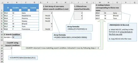
Demonstrates the search condition that we have established. In this example we are looking for all the rows where Gender = M
The equivalent COUNTIF function has been shown below to return the number of rows found with this condition is 3
Step2:
Establish an array formula =IF($B$2:$B$8=$B$11,ROW($B$2:$B$8)).
This is an array formula and uses an extension of the regular IF function. It compares the values in the array B2:B8 with B11 and return the results of the comparison as an array of values. When comparison is true, the result is the ROW() number, else FALSE (because no value provided when comparison is false).
To understand this further, you can start with the simpler IF formulaes as below and experiment with different options in the value_if_true and value_if_false and understand the results
`IF(B2=B11,ROW(B2),)'
`IF(B2=B11,ROW(B2),"mismatch")'
Now try the same by changing B11 to F and then see what happens to the results.
Step 3:
Here we are using the SMALL function to return the nth smallest value in an array. However the trick here is to change the nth value on each row. So the first row should show the smallest value in the array F2:F8, the second row should return the 2nd smallest, and the third row should return the third smallest value.
So we use the ROW()-1 to get the corresponding nth variable setup, and the rest is easy.
Step 4:
At the end of step 3 we have the number of rows where our search condition is satisfied. Now in this step all we need to do is use the INDEX function to extract the row values corresponding to these row numbers.
To achieve this, first select cells M2:O2, press F2 and your cursor will be located in cell M2. Enter the formula INDEX($A$1:$C$8,J2,0) and press Ctrl + Shift + Enter together for this to work as an array formula. The 0 in this formula forces to return the entire row instead of values from a specific column from the range A1:C8.
Now Select M2:O4 and press Ctrl+D to copy the formula in the top most row to the cells below.
BINGO!
Post your comments if you need clarifications and I will be more than happy to clarify.
I have used a number of simplifications and broken down the steps to explain the functioning. All of these formulaes can be combined together to achieve the same results in one go.
Also another simplification: choosing to enter the formulaes in the exact number of rows, however, when you do not know the number of rows that will be returned by the search condition, then you can make the final result array as large as the original data set range to potentially cater for if all the rows are returned. You can also add error handing in each of the formulaes to show blank rows when the number of rows returned is smaller than the result area. Hope this makes sense!


