5

In an Excel worksheet:

Column A is all filled with random text values (e.g., words / sentences) that need to be updated.

And columns B and C contain strings that specify the changes that need to be made to column A. Column B is filled each cell with the old text and column C with the new text, each line corresponding to each other, this is, text in B1 need to be substituted by text C1, B2 to be changed for C2 text. In column B one of the things to substitute is a ".

There are no repeated values in column B. Cells may be repeated in column C, though. The substitutions must obey the order in which they were written. And column D is the result.

Each cell from column A needs to pass through this substitution from B1-C1, B2-C2, B3-C3, etc., until the end of the substitution commands in columns B-C. So, before giving the final result, the text from column A will change several times, and only will show result in column D after all changes.


Example:

Cell A1: Hello!
Cell A2: How are you "John"?
Cell A3: "Nice! thanks"
Cell B1: !                           Cell C1: &
Cell B2: &                           Cell C2: .
Cell B3: "                           Cell C3:    (empty)
Cell B4: ?                           Cell C4: #
Cell B5: Nice. thanks                Cell C5: Fine, THANKS.

So Cell A1, which is Hello!, will be changed by B1-C1, so will be Hello&. Then will change B2-C2 with changes made to the temporary result Hello& so will be Hello..  Then will change B3-C3 and then will do B4-C4 and then B5-C5, and nothing will happen because " doesn’t exist in Hello..

After this, result D1 is Hello..

Then it will do A2 changes B1-C1 (nothing to do), then applied to this will do B2-C2 (nothing to do), then B3-C3 which will result as How are you John? (i.e., the quote characters will be removed), then will do B4-C4 which will make How are you John#, and then B5-C5 which has nothing to be done in here.

So result D2 is How are you John#.

The same way, A3 value "Nice! thanks" will have change from B1-C1 at first, becoming "Nice& thanks", then B2-C2 becoming "Nice. thanks", then B3-C3 becoming Nice. thanks (again, the quotes will be removed), then nothing to do in B4-C4 and then B5-C5 will make it become at last Fine, THANKS in D3.


Results:

D1: Hello.
D2: How are you John#
D3: Fine, THANKS.

What would be the formula in column D for doing this multiple substitutions in a row obeying the line order written in columns B and C, allowing column B-C to have more than 300 lines? (I would like a purely formula based-solution, rather than VBA, if possible.)
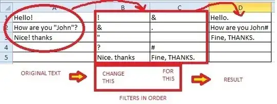
sample data from above with processing flow illustration

Joao
  • 493

3 Answers3

4

I'd hoped for a clever way to do this using a single array formula, but couldn't find one (I'd love to be proved wrong!) I think the only way to do it with a single formula per line of input is to nest SUBSTITUTE functions, as per @G-Man's answer. Sadly, this strategy won't work for 300 substitutions, as Excel has a limitation that functions can only nest 64 levels deep (or 7 before Excel 2007).

Hence I think you'll need helper columns (which you can always hide if it helps with presentation). The method below uses simpler formulas than G-Man's. It uses a few more helper cells than his: one column per input string × one row per substitution plus one:

  • Starting with the worksheet laid out as per your example, insert a blank row at the top of the page. Select cells F1:H1, type the formula =TRANSPOSE(A2:A4) and press Ctrl+Shift+Enter, so it gets entered as an array formula. You should see curly braces appear around the formula, and the cells should fill with your input strings.

  • In cell F2, enter the formula =SUBSTITUTE(F1,$B2,$C2). Copy this formula across and down to fill all of F2:H6. Your desired output will appear in F6:H6.

  • To get your output back to column D, select D2:D4 and enter the formula =TRANSPOSE(F6:H6). As before, Ctrl+Shift+Enter so it works as an array formula.

This should scale easily for more input strings (use more columns) or substitutions (use more rows); just adjust the ranges accordingly. If you don't actually need the input and output in columns, you can easily do without the TRANSPOSE formulae too; just enter your input in the top row to start with.

JRI
  • 907
2

You can do what you describe/illustrate with

=SUBSTITUTE(SUBSTITUTE(SUBSTITUTE(SUBSTITUTE(SUBSTITUTE(A1, B$1, C$1), B$2, C$2), B$3, C$3), B$4, C$4), B$5, C$5)

If you put the above into cell D1 and drag/fill down, the A1 will update to A2, A3, etc., but the substitute string parameters (B$1, C$1, B$2, C$2, etc.) will not change.  I believe that it’s obvious that this performs the B1 → C1 substitution on A1, then performs the B2 → C2 substitution on the result from the first substitution, then performs the B3 → C3 substitution on the result from the second substitution, and so on.

This is awkward for five substitutions, and rapidly becomes unwieldy for more.  If you may want to do many substitutions (say, up to 312), use helper columns:

  • Set AA1 to

    =SUBSTITUTE(A1, INDEX($B:$B, COLUMN()-COLUMN($Z1)), INDEX($C:$C, COLUMN()-COLUMN($Z1)))
    

    This is equivalent to =SUBSTITUTE(A1, B1, C1), but it gets the B1 and C1 values dynamically by taking the column number (AA → 27) and subtracting 26 (the column number of column Z), and using the result (1) as the row number in the B and C columns.

  • Drag/fill AA1 to AB1, so it becomes

    =SUBSTITUTE(B1, INDEX($B:$B, COLUMN()-COLUMN($Z1)), INDEX($C:$C, COLUMN()-COLUMN($Z1)))
    

    and change B1 to AA1, so it becomes

    =SUBSTITUTE(AA1, INDEX($B:$B, COLUMN()-COLUMN($Z1)), INDEX($C:$C, COLUMN()-COLUMN($Z1)))
    

    This is equivalent to =SUBSTITUTE(AA1, B2, C2), which is equivalent to =SUBSTITUTE(SUBSTITUTE(A1, B1, C1), B2, C2).

  • Drag/fill AB1 to LZ1.  This will be the result of A1 with all the substitutions from B1:C1 to B312:C312 applied (because L is the 12th letter, and 12×26 is 312).
  • Set D1 to =LZ1, to reflect the result of all the substitutions.
  • Drag/fill D1 and AA1:LZ1 down as far as you have data in column A.
2

While I know you were after a formula-based solution, I thought a VBA version would be helpful for reference, as I couldn't find one online:

Function MULTISUB(aString As String, oldVals As Range, newVals As Range) As Variant
    oldW = oldVals.Columns.Count
    oldH = oldVals.Rows.Count

    If (oldW = newVals.Columns.Count) And (oldH = newVals.Rows.Count) And (oldW = 1 Or oldH = 1) Then
        MULTISUB = aString
        For i = 1 To oldVals.Count
            MULTISUB = Replace(MULTISUB, oldVals.Cells(i), newVals.Cells(i))
        Next i
    Else
        MULTISUB = CVErr(xlErrRef)
    End If
End Function

For your example, you would enter =MULTISUB(A1,$B$1:$B$5,$C$1:$C$5) in cell D1 and copy it down to D3.

The function takes a string and two ranges. It searches the string for the values in each cell in the first range, and replaces them with the values of the corresponding cells in the second range. If the two ranges aren't the same shape and size, it returns #REF.

JRI
  • 907