@Tee, in case you are still around, I'm posting an answer to your question. It took quite a while to clearly understand the problem you're facing, and I'm still not sure I have it exactly correct.
So let me state the problem that I have solved, and I hope to give you enough information to modify the solution if my understanding of your problem is incorrect.
Problem: You want to calculate a running sum of 35/36ths of each of the numbers that start in G17 of your spreadsheet and continue beyond AP17. The tricky part is that once there are 35 terms in your sum, the start of the range must move to the right (i.e H17, I17 etc.), as the formula is filled to the right.
The following discussion will show how to calculate the sum, and the final formula will be multiplied by 35 and divided by 36.
Solution: To calculate the sum, a formula like this is required:
=SUM(INDEX(reference,row_num,[column_num]):INDEX(reference,row_num,[column_num])
The "reference" form of INDEX() can be used to return a cell reference, and here, the first INDEX() calculates the start of the range to be summed, while the second INDEX() calculates the end of the range.
The sum starts with G17 (column 7), for all columns less than column AP (column 42). Beginning with column AP, the starting cell moves one column to the right as the formula is filled to the right. So the first INDEX() is:
INDEX($17:$17,1,IF(COLUMN()<42,7,COLUMN()-34))
As an example, in column AP, the sum range starts with H17. Column 42-34 = 8 = column H.
The end of the range to be summed is just the current column. So the second INDEX() is:
INDEX($17:$17,1,COLUMN())
Now the sum is:
SUM(INDEX($17:$17,1,IF(COLUMN()<42,7,COLUMN()-34)):INDEX($17:$17,1,COLUMN()))
And the final formula is:
=35*(SUM(INDEX($17:$17,1,IF(COLUMN()<42,7,COLUMN()-34)):INDEX($17:$17,1,COLUMN())))/36
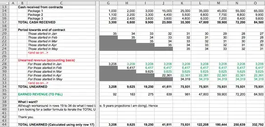
A portion of your spreadsheet with the calculation is shown in the picture below. Please comment if you are still visiting here. Best regards.
