Manipulate data in Excel to order results per a certain column

Question

I want to make the information in some columns (but not all) displaying in rows, please see below an example.

This is what I have (unfortunately this doesn't allow extra spaces so everything is unaligned, please try to imagine all aligned):

Patient     Visit 1     Visit 2     Visit 3     Visit 4(…)

1           22Dec       12Jan       03Feb    
2           3Jan        03Feb       01Mar
3           10Dec       03Jan       23Jan   
(…)

(etc, long database with hundreds of patients)

This is how I want it to look like:

Patient     Visit type      Date

1           Visit 1         22Dec
1           Visit 2         12Jan    
1           Visit 3         03Feb   
2           Visit 1         23Jan   
2           Visit 2         (…)   
(…)

It doesn’t involve any calculation, it’s just data manipulation, basically ordering the visits per patient, but I am not sure of any function that does this, tried pivot table but doesn’t seem to do it quite like this… Any suggestions? If there are no formulas, no buttons, etc, perhaps can you suggest a macro?

Many thanks!

score 1 · Answer 1 · answered Feb 28 '18 at 17:24

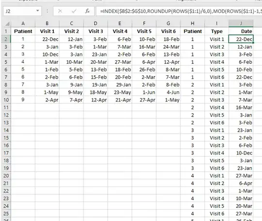
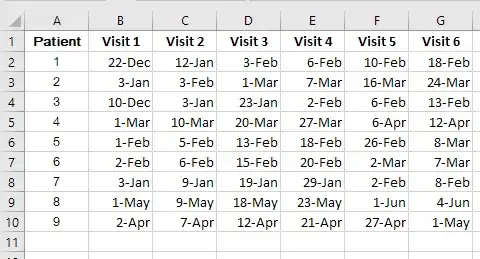
With data like:

In H2 enter:

=ROUNDUP(ROWS($1:1)/6,0)

and copy downwards. In cell I2 enter:

=INDEX($B$1:$G$1,MOD(ROWS($1:1)-1,6)+1)

and copy downward. In J2 enter:

=INDEX($B$2:$G$10,ROUNDUP(ROWS($1:1)/6,0),MOD(ROWS($1:1)-1,5)+1)

and copy downward:

NOTE:

The 6 in these formulas corresponds to the number of visits in the source table. Adjust to suit your needs.

score 0 · Answer 2 · edited Feb 28 '18 at 18:06

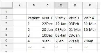
It was not clear to be if you want a continuous transformation, or just to transform your data once. If you just want to transform you data once, here’s a suggestion: Let’s imagine this is your data now:

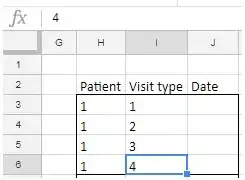
As you have a maximum of 4 visits per patient, build manually the rows for the first patient, like this:

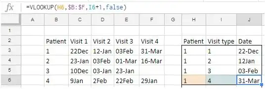
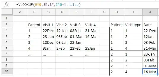
For the date column, apply the VLOOKUP, searching the column according to the visit type:

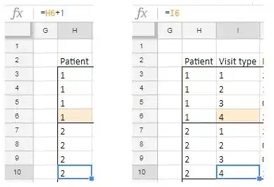
Now build manually the rows for the second patient, but now with some formulas you will be able to push down:

For the date column, just push down what you have from patient 1:

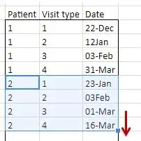
Now, select the all block of patient 2 and push down:

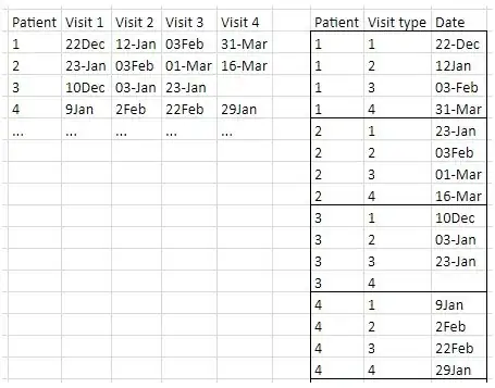
Even when there’s no date, it will work

Will this suit you?

score 0 · Answer 3 · edited Mar 03 '18 at 18:09

My approach uses a Two Way Lookup technique, just like one of the answers above.

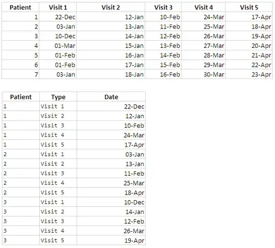
See the pictures below, which show the sample data in the first table, then the list of patients, visit number and date, all in the desired order, in the second table.

Here are the formulas to get the:

Patient list: in Cell A10, =INT((ROW(A1)-1)/5)+1

Visit Type list: in Cell B10, ="Visit"&INT(MOD(ROW(A1)-1,5))+1

Date List in Cell C10, =INDEX($B$2:$F$8,MATCH(A10,A$2:A$8,0),MATCH(B10,$B$1:$F$1,0))

Drag all 3 Formulas down, as far as required.

I do hope this helps you.

Manipulate data in Excel to order results per a certain column

3 Answers3