I'd approach this just a little different than Bandersnatch (although the principle is the same).
Since you've already got your invoice data in an Excel Data Table (which is good), here's what I would do:
1) Create an XY/Scatter Chart using your Data Table for the primary data series, with:
x axis = Date
y axis = Amount
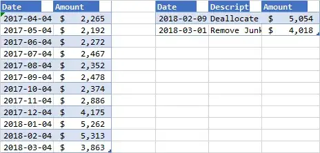
2) Create a second table for your event data. You'll need 3 columns Date, Amount, Description.
3) The Date and Description columns you can pull from your current table. The simple way to do this would be to add your Event series using Date as your x-axis, and then using a single helper value (e.g. 0 or 6000) for your y-axis. This would align all of your points vertically, but not on your line.
What I would do is to interpolate the y-axis value for your date and use that as your y-axis series. Using a combination of structured names (since you're using Data Tables), and the FORECAST.LINEAR, MATCH, AND OFFSET formulas, your Event Table Amount Column formula would be something like this:
=FORECAST.LINEAR([@Date],
OFFSET(tbl_Overall_Price[[#Headers],Date]],
MATCH([@Date],tbl_Overall_Price[Date],1),1,2,1),
OFFSET(tbl_Overall_Price[[#Headers],[Date]],
MATCH([@Date],tbl_Overall_Price[Date],1),0,2,1))
4) Then, add your Event data series to your chart and format to taste.
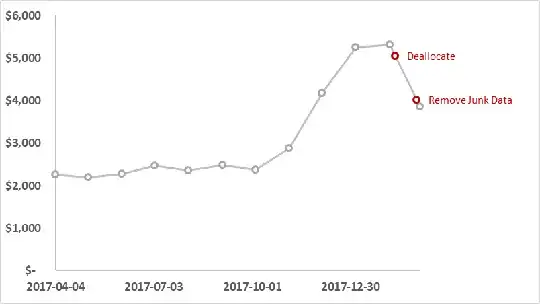
5) Now that Excel 2016 allows you to use a cell range for Data Labels, just use your Description column for your labels.


