As other Users have explained, the only way to have a "linked" cell that auto-updates its format when the source cell's format changes is to use VBA.
However, if the only thing you wish to do is directly mirror a source cell without any other calculations (e.g., you just want to do =A1 but also have the formats update), there is a way to make it look like that's what's happening.
Just four simple steps:
- Select the source range
- Copy
- Select the top left cell of the destination range
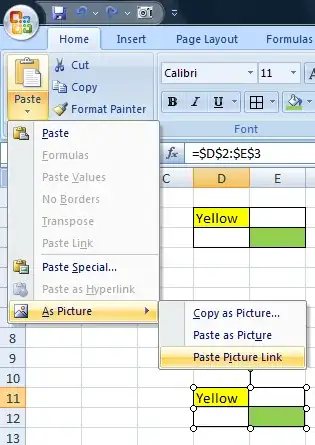
- Paste as a Picture Link (
Home → Clipboard → Paste → As Picture → Paste Picture Link)
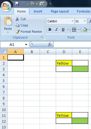
The following screenshots show how to create a picture link at D11 linked to D2:E3 and how it looks when the picture is deselected:
Notes:
Unfortunately you can't actually use the values from the picture for any further calculations.
However, there is a work-around for this. Just directly link the cells underneath the picture to the source as well. In my example above, you would enter =D2 into cell D11 and ctrl-enter/fill/copy-paste that formula into D11:E12.
The only issue with this work-around is that blank source cells will show through the picture as 0s if the source cell's fill is set to No Fill.
To work-around this 0 issue, either set the destination cells' font colour to the fill colour (use white for no fill), or, if you actually require the destination to actually be "blank", use the formula =IF(D2="","",D2) instead of =D2.

