Organizing data in excel after breaking it up with text-to-column

Question

I have a messy spreadsheet where each row has a name then a cell with a list of tags (like "Jane Smith | tag 1, tag 2, tag 3"). I used text-to-column to break the list up into multiple cells, like this:

Name       | Tags
Jane Smith | tag 1 | tag 2 | tag 3
John Doe   | tag 1 | tag 3 | <nothing>

But the problem is that the lists I broke up were not the same length (since not every person was tagged with the same things), so not every "tag 3" is in the same column. Ideally I'd love to end up with spreadsheet that looked like this

Name       | Tag 1 | Tag 2 | Tag 3
Jane Smith | TRUE  | TRUE  | TRUE
John Doe   | TRUE  | FALSE | TRUE

Is there an easy way to get to this? Any help would be much appreciated.

Edit: here's some example data: https://www.dropbox.com/s/u6vpgw0dzgjaz8n/sample_tag_data.xlsx?dl=0

Answer 1

I would unpivot the data into a normal list, then create a proper PivotTable from that.

1. Unpivot

Thankfully, newer versions of Excel include PowerQuery that makes it much easier to unpivot than it used to be (as shown in the "Possible duplicate" link in the comments). I used your sample data spreadsheet.

• (In an empty cell) Data menu, From Table/Range, Select your table and check "Has headers"
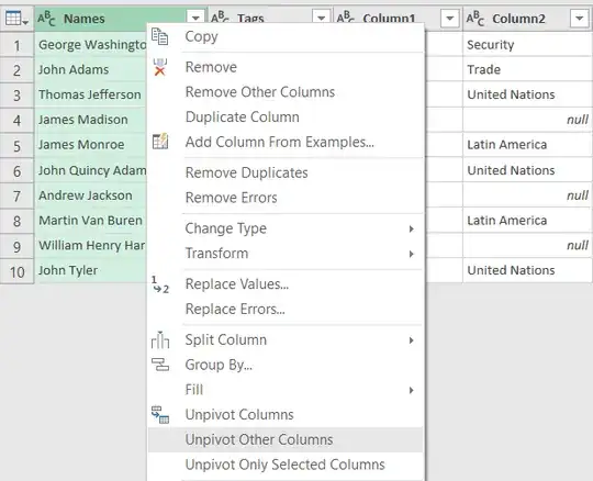
• In the Power Query Editor, right-click the Names column and select "Unpivot other columns" (or select all tags column and pick Unpivot Only Selected Columns).
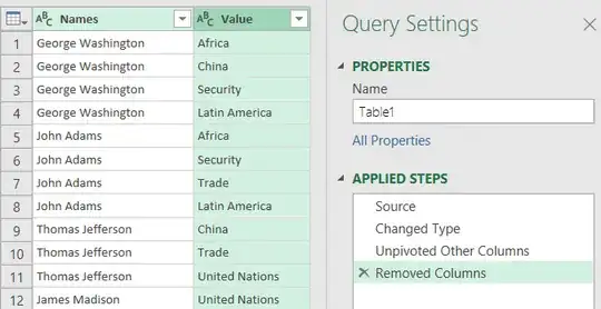
• Right-click Attribute Column and select Remove Columns
• Right-click Value column and select rename to "Tag"
• Click Close & Load To and select "PivotTable Report"

2. (re-)Pivot

Power Query has added a query to your spreadsheet and we have an empty PivotTable linked to it.

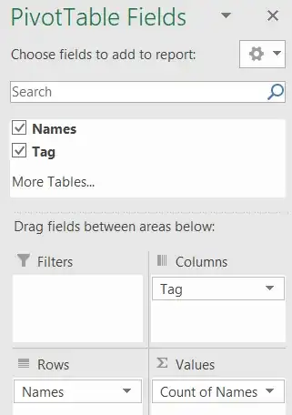
• Select a cell in the PivotTable to display the Pivot Panel.
• In the Pivot Panel, build the pivot by adding the Name field as Row Label, Tag as Column Label, and Tag as Values.
• Adjust styling as desired.

PivotTables usually shows sums or counts instead of "TRUE" but it also provides useful totals and many ways to arrange and format your data. To answer your question exactly you could remove totals and set a custom number format to show "TRUE", but I would not recommend it:

• Right-click in the PivotTable, Options, Totals tab, uncheck all. OK.
• In the Pivot Panel, click the count in values select Value Field Settings, click Number format, select Custom, type "TRUE".

Finally, Power queries and Pivot Tables also make it easy to "Refresh data" if you update your source table without having to redo these steps each time.