2

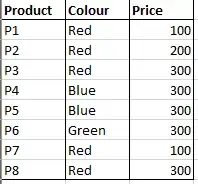
I have a table with some data that is similar to the table below:

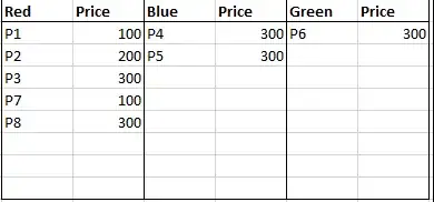
enter image description here

I would like to display a table on the right of this table to show each colour product in its own column:

enter image description here

The worksheet would therefore look something like this:

enter image description here

  • When update the table on the left, i would like the table on the right to update automatically (including adding and removing rows).

After googling around, i found a few examples but none of them seem to do what i would like to do:

  • The data can be filtered but i am not sure if filtering can be done with multiple tables.

  • I tried a Pivot table but could not get it to show anything other than totals. Maybe i did something wrong but the only view i could get was totals and sums of the values - i could not create the second table using a pivot table.

  • Is it possible to do this with VLookup but not have blank entries where there is no match?
ziggy
  • 353

2 Answers2

0

Assuming the Product:Colour:Price table is located at A1:C9, and the Red:Price:Blue:Price:Green:Price table is located at F1:K9 :

In F2 put :

=IF(ROW()=2,IFERROR(INDEX($A$2:$A$9,MATCH(F$1,$B$2:$B$9,0)),""),IFERROR(INDEX(OFFSET($A$2:$A$9,MATCH(F1,$A$2:$A$9,0),0),MATCH(F$1,OFFSET($B$2:$B$9,MATCH(F1,$A$2:$A$9,0),0),0)),""))

In G2 :

=IF(F2="","",IFERROR(INDEX($C$2:$C$9,MATCH(F2,$A$2:$A$9,0)),""))

then drag both until K9. Please if it works/stuck/error.. ( :

Hope it helps.

p._phidot_
  • 1,273
  • 1
  • 8
  • 14
0

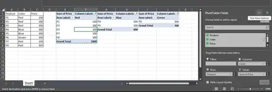
You could achieve this using three pivot tables (depending on how many colors you have) and filter each with the corresponding color.

It's not exactly formatted like your example, but it's the easiest without using complicated formula and this is fully automated. You still need to Refresh All if you update the source table, though.

Note: this is taken from Excel 2021, but should work with previous editions.

Screenshot of the example table and the pivot tables

  1. Create the first pivot table
  2. Put the Color column for the Column
  3. Put the Product column for the Row
  4. Put the Price column for the Value
  5. Remove Grand Total column - you cannot remove Grand Total row
  6. Set the first color filter (for example: Red)
  7. Copy paste the pivot table
  8. Set the other color filters
Vylix
  • 1,935