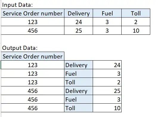
Service Order Number =INDEX($A$2:$A$100,INT(ROW($A3)/3))
- where
$A$2:$A$100 is the service order numbers range.
- where
$A3 is Not used to reference a cell's value. Leave $A3 row reference relative.
Row Headings (Middle Column) =INDEX($B$1:$D$1,MOD(ROW($A3),3)+1)
- where
$B$1:$D$1 is the column headings.
Row Values =INDEX($B$2:$D$100,INT(ROW($A3)/3),MOD(ROW($A3),3)+1)
- where
$B$2:$D$100 is the delivery/fuel/toll data range.
Copy all three formulas to consecutive cells on the same row:
ServiceOrderNumber | RowHeadings | RowValues
If these formulas live on a different sheet than the data, be sure to qualify the range with the sheet name: Sheet1!$A$2:$A$100
Select All Three Formula Cells. With all three selected, copy drag down together (this way all three formulas are copied down together instead of one at a time).
Why it works:
- The
$A3 cell reference will increment in row value for each row the formula is copied drug down.
ROW of this incremented row reference will provide numbers: 3,4,5,6,7,8,...
INT of division by 3 will cause every 3 rows to act as one: 1,1,1,2,2,2,...MOD of 3 will will cycle through columns: 1,2,3,1,2,3,...
