I have a table of measurements, with each data point being measured multiple times.
I would like to create a PivotChart which displays the average value and uses the value's standard deviation as error-bars.
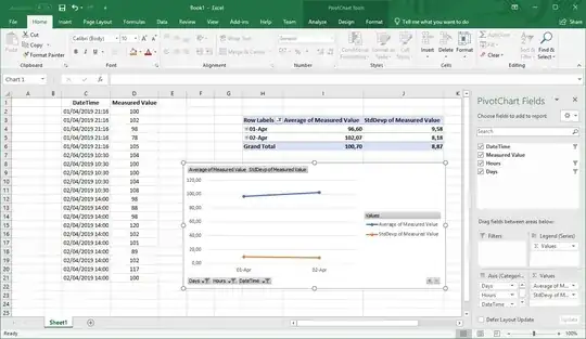
This is what I have so far:
- My DataTable has one category column (Date & Time) and one value column.
- I have a PivotTable which generates me the average value, and it also generates the standard deviation
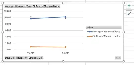
- My chart currently shows the average and the stdDev as individual data series.
I would like to have the stdDev series (orange) not in the graph, but have the average series (blue) to show error bars. These error bars should have the size of the stdDev values.
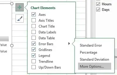
I can find the error-bar option, but I don't see a way to assign the (computed) StdDev as magnitude.
The options given, only use the standard deviation across the values of the pivotTable.
This is not what I want.
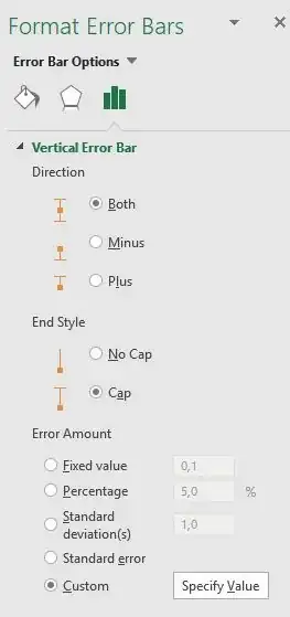
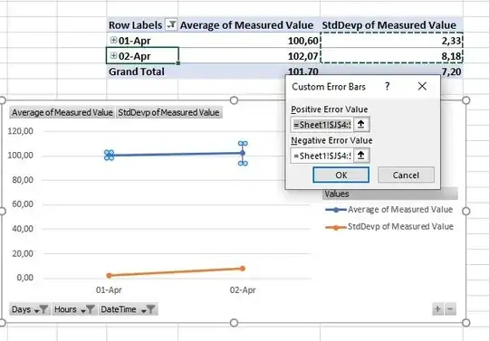
But if I go to the advanced options:
I can also only find a method to specify a fixed custom value.
While the field seems to allow for a table-range to be selected, I can only do so for a specific section. i.e. I can select the according values in the pivot table and get my graph:
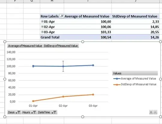
The error-bars are now as I want them, but any change of the pivot table structure, i.e. adding new dates, looses the connection:
I want the error-bars to always use the computed value of the same row - can this be done?
( And I also want to hide the orange series, but that is secondary. )
