0

Is it possible to 'superimpose/show' data from a similarly shaped matrix over a range heatmap, instead of simply showing/hiding the underlying heatmap data?

The question could also be rephrased differently: Is it possible to generate a heatmap on any given range (say A1:C3) based on a data range elsewhere on the sheet (e.g. F1:H3)? If yes, one could make visible the A1:C3 values over the heatmap.

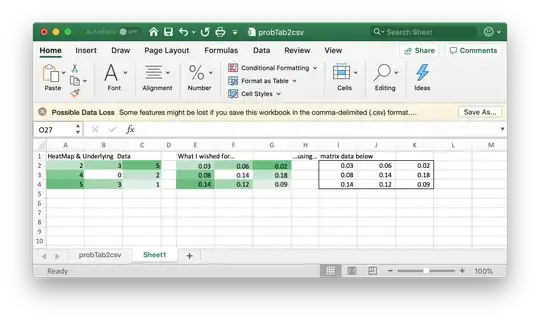
The goal here is simply to get the heatmap to show more information and following (very basic) screenshot will clarify what I am looking for:

Regular heatmap & custom one showing data from a different range

The left one is an actual standard one built from the data behind the coloured background, while the one I am looking for (in the middle) is built using the same data than the left one for the heatmap itslef, but showing/superimposing a set of values from the range at its right (this was done using a picture paste).

Once again, the idea is to convey 2 times more information: one set through colour, and another one, different, using data from another range.

Obviously useful when the two data sets are related in some way.
Giacomo1968
  • 58,727

1 Answers1

0

The best solution I could think of at this time is to use Excel's Linked Picture utility. Here is how it works (based on your example - adapt as needed):

  1. Insert 4 columns right of column C
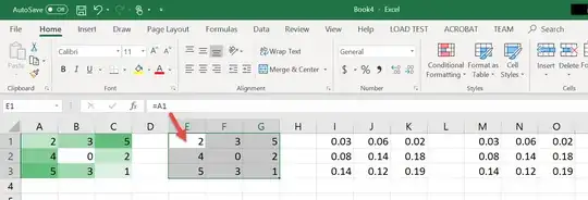
  2. In cells E1:G3 link them with a formula to cells A1:C3 (e.g. in E1 write formula =A1 and so forth

enter image description here

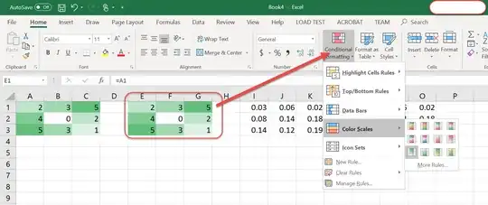
  1. In cells E1:G3 apply the same conditional formatting as in cells A1:A3. (unless you have another purpose, you really don't need conditional formatting for A1:C3)

enter image description here

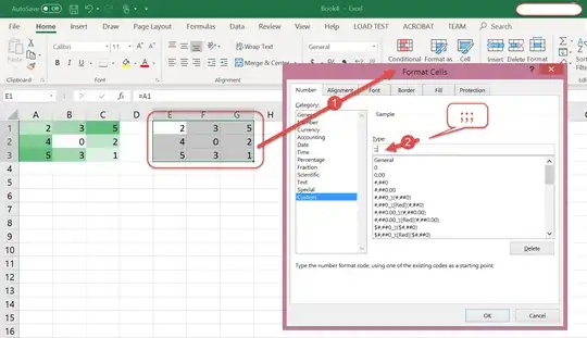
  1. In cells E1:G3 format cells with custom type ;;; (note: conditional formatting is missing in E3:G3 in picture below because I took screenshots out of order)

enter image description here

  1. This is what your worksheet should look like at this point

enter image description here

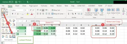
  1. Select and copy cells M1:O3, go to cell E1 and paste special Linked Picture.

enter image description here

That's It.

Now you can alter values in cells A1:C3 to change the conditional formatting in E1:G3 and you can alter value in cells M1:O3 to change values in E1:G3. If E1:G3 is the output you want to see, you can move A1:C3 and M1:O3 somewhere else - they are now simply used for inputs. I did not use the cells in I1:K3 in your example because they weren't needed (and obviously you used them just as an example. I wish this could be done more elegantly but this seems to be it given Microsoft Excel limitations. What you are asking would be a great feature I can see being useful.

Brian
  • 1,085