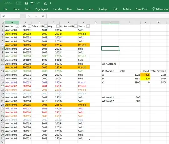
I'm struggling to sum the right values. It looked quite easy at first, but the more it try it the more complicated it seems to be. An example of my data is in an image below.
My data consists of sellinglots from an auction company, in the example there are 3 different auctions (auction01, 02 and 03) in the same table. Column B contains the LotID, D = quantity that I try to sum, E = customerID and F = status (sold or unsold).
What I try to do is sum the unsold quantity with the following criteria:
- qty per CustomerID
- only distinct LotID
- only unsold qty after all auctions. (e.g. lotID 900002 and 900005 are never sold, while 900013 is unsold at auction02 but sold at auction03 so I don't want to sum it.)
I got quite close, but I can't seem to get the last criteria implemented.
The results I want are in Cells J14 and J15, my 2 attempts for customer A are in cell I20 and I21.
Attempt 1:
=SUM(IF(FREQUENCY(IF(Table1[CustomerID]=H14;IF(Table1[Status]=J13;MATCH(Table1[LotID];Table1[LotID];0)));ROW(Table1[Qty])-ROW($D$2)+1)>0;Table1[Qty]))

Attempt 2:
=SUMPRODUCT(IFERROR((Table1[Status]&Table1[CustomerID]=J13&H14)/COUNTIFS(Table1[LotID];Table1[LotID];Table1[Status];J13;Table1[CustomerID];H14);0);Table1[Qty])

