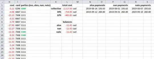
I'm using Excel for the accounting purposes of a group venture, to keep track of our expenses, costs, payments, and balances.
- Details of each expense are stored in columns
A:J - Total costs and balances are stored in columns
K:M - Payments and dates are stored in columns
N:S
Generally speaking, I'm responsible for 34% of the cost of most expenses, whereas each other party is responsible for 22% of the cost of most expenses. This is the case for the majority of expenses.
However, there are a few expenses that I would like to split only between specific parties – J2, J9, and J10 – which are emphasized by a green, bold font in the screenshot above.
Understanding the parties column:
1111(me, alex, nan, nate)1100(me, alex)1000(me)0101(alex, nate)- et cetera
I'm not sure how to go about this, therefore I have a few questions:
Is there a formula to ignore certain values in a row based on other values in the same row? For example, is there a way for the collective total cost formula,
=SUM(H:H), to ignoreH2,H9, andH10, other than something like=SUM(H3:H8,H11:H99999)?Conversely, is there a formula to select every value in the
Hcolumn whose value in theJcolumn is equal to1100for example?
