Optimizing item position using in a warehouse excel formula

Question

I currently am in need of an excel formula or way to do this simple optimization to sort items by popularity.

Context:

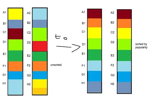
The image is a top-down view of course, each square is a product we sell, and the color represents popularity and the two columns is because it's an alley. The popular items have to be at the top because they are the closest to the packaging machine which makes it significantly faster to move if it's closer while non-popular items that don't get shipped too often should be further away. The popularity varies throughout each day too.

Currently I print out the (left side of the image) and sort and move each item manually to the top, but it's a tedious process because it's a rather busy warehouse so it takes time to move, so I only move the most popular two products to the top.

Problem:

So I want to make an excel sheet that tells me to move item [RED] from C1 to A1, and D2 to A2, for [ORANGE] from F1 to B1, and F2 to B2 and so on... I have a column A for product code (basically the colors), B for location (like A1, A2, ..., in the image), C for popularity (The color, aka how much is expected to be sold today), and D for stock balance (Not necessary, but could be added for context)-

My current solution is to copy the columns article, location and popularity, then sort by popularity using AZ sort-thing in Excel which gives the order I'm looking for, but then I have to manually write Move To, and also the new sorted copy has to say "Move from" cause it shows the most popular item's location, but I want to move that popular item TO the first location. And also the warehouse is huge with > 500 products so doing it all manually and accounting for every alley is very tedious.

I might be explaining the problem bad but please bear with me.

Here is a sample of redacted data:

NOTE: The image is not to scale and the colors are supposed to take up same amount of space, so ignore that and assume they are just equal sized cells.

Answer 1

Essentially you want to calculate the rank of each product within each alley (aisle).

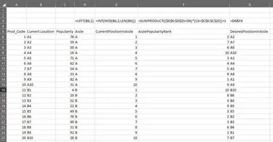
I created some dummy data in columns A, B and C.

In Column D, I extracted the part of the Current Location that indicates which aisle the product is in. In my data, I used this formula, but you may need something slightly different depending on the structure of your location codes:

=LEFT(B6,1)

In column E, I extracted the part of the Current Location that indicates which position that product is currently in in the aisle. Actually I realised this step is not strictly necessary, so you can skip it if you want, but it may be useful for comparison.

=INT(MID(B6,2,LEN(B6)))

MID will extract some text starting at position 2 (i.e. after the letter) and continue to the end of the location code. INT will convert it to a number.

F is the important column and is where we calculate the rank of the popularity within each aisle.

=SUMPRODUCT(($D$6:$D$25=D6)*(C6<$C$6:$C$25))+1

Now that I have the desired position in the aisle, I can reconstruct in column G the desired position in the same format as the current location.

I'm sure your solution will differ slightly because the structure of your location code will define how you need to extract the Aisle-indicator (which is important in calculating the rank), but I hope you will be able to extrapolate from this to solve your issue.

EDIT1:

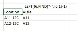
Since you mentioned that the aisle in the location code A11-12C would be A11, then you presumably want to extract the aisle from that text as being everything before the hyphen. For that, this formula should do:

=LEFT(I6,FIND("-",I6,1)-1)

EDIT2:

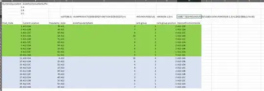
So according to your description of the Location code, this should do the trick:

In column D, extract the Aisle indicator:

=LEFT(B8,3)

Column E is as specified above (SUMPRODUCT).

Since you have a pattern of A-B-C before incrementing the position from 11 to 12 to 13 etc, you need to distinguish between these groups, then the position within these groups. That's what columns F and G are for.

F assigns a number to each group of three positions, starting at rank=1 and continuing from there:

=ROUNDUP(E8/3,0)

G assigns a repeating 1,2,3 within each group:

=MOD(E8-1,3)+1

To convert the 1,2,3 position within each group back to A,B,C, I created a small lookup table in the top-left of the image above. This is so I can use VLOOKUP:

=D8&"-"&10+ROUNDUP(E8/3,0)&VLOOKUP(MOD(E8-1,3)+1,$A$2:$B$4,2,FALSE)

You can probably do away with some of those intermediate columns by nesting the functions appropriately.