Transposed counts for many columns

Question

The input:

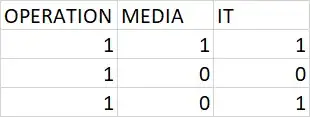
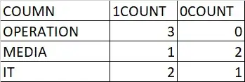
I have to get the count of the number of '1' and '0' in each column like this:

Is there any way in Excel/macro to do this?

Answer 1

Excel Power Query solution

Result:

---

For pros - full procedure:

let
    Source = Excel.CurrentWorkbook(),
    #"Expanded Content" = Table.ExpandTableColumn(Source, "Content", {"OPERATION", "MEDIA", "IT"}, {"OPERATION", "MEDIA", "IT"}),
    #"Removed Columns" = Table.RemoveColumns(#"Expanded Content",{"Name"}),
    #"Unpivoted Columns" = Table.UnpivotOtherColumns(#"Removed Columns", {}, "Attribute", "Value"),
    #"Grouped Rows" = Table.Group(#"Unpivoted Columns", {"Attribute", "Value"}, {{"Count", each Table.RowCount(_), type number}}),
    #"Pivoted Column" = Table.Pivot(Table.TransformColumnTypes(#"Grouped Rows", {{"Value", type text}}, "en-US"), List.Distinct(Table.TransformColumnTypes(#"Grouped Rows", {{"Value", type text}}, "en-US")[Value]), "Value", "Count", List.Sum),
    #"Replaced Value" = Table.ReplaceValue(#"Pivoted Column",null,0,Replacer.ReplaceValue,{"Attribute", "1", "0"})
in
    #"Replaced Value"

---

For others - detailed steps.

Select your input data table (including headers).
Insert -> Table

OK

Click on the double arrows next to "Content"
Uncheck Use original column name as prefix

OK

Right-click on column "Name" -> Remove

Select whole table
Transform -> Unpivot Columns

Home -> Group By

OK

Select column "Value"
Transform -> Pivot Column
As Values Column select "Count"

OK

Select whole table
Transform -> Replace Values
Fill in like this:

OK

Home -> Close & Load

Answer 2

If we say that the columns start at "D1" and we print to "A3", it could looks something like this:

Sub countAndTranspose()
Dim section As Range, count As Range, entry As Range, sectionPrint As Range

Set section = Range("D1", Cells(1, Columns.count).End(xlToLeft)) 'All headers
For Each entry In section
    Set sectionPrint = Cells(Rows.count, 1).End(xlUp) 'Last row in "A"
    Set count = Range(Cells(entry.Row + 1, entry.Column), Cells(Rows.count, entry.Column).End(xlUp))
    sectionPrint.Offset(1).Value = entry.Value 'Print header below last row in A
    sectionPrint.Offset(1, 1).Value = WorksheetFunction.CountIf(count, 1) 'Print sum of 1
    sectionPrint.Offset(1, 2).Value = WorksheetFunction.CountIf(count, 0) 'Print sum of 0
Next entry

End Sub

We start with defining our range of columns, starting at "D1" and going to the far light of the row.
Then we loop through this range, picking where to print the column name (A3 and down should be EMPTY)

Answer 3

Below the column entries of OPERATION, MEDIA and IT please enter two formulas:

COUNTIF ( A2:A10, 1 ) for ones
COUNTIF ( A2:A10, 0 ) for zeroes.

Copy the formulas below MEDIA and IT.

Answer 4

For a non-VBA solution, you can take advantage of LET if you have Excel 2016 or Microsoft 365. This will work on Excel for Mac as well (unlike Power BI).

=LET( array, A1:E4,
       hdr, INDEX( array, 1, ),
       rSeqBody, SEQUENCE( ROWS( array ) - 1 ),
       cSeq, SEQUENCE( 1, COLUMNS( array ) ),
       body, INDEX( array, rSeqBody + 1, cSeq ),
       onesCount, MMULT( TRANSPOSE( SIGN( rSeqBody ) ), body ),
       t1s, IFERROR( INDEX( TRANSPOSE( hdr ), TRANSPOSE( cSeq ), {1,2} ), TRANSPOSE( onesCount ) ),
       t10s, IFERROR( INDEX( t1s, TRANSPOSE( cSeq ), {1,2,3} ), ROWS( body ) - TRANSPOSE( onesCount ) ),
       t10s )

This is an example application:

Where the input is the array, including the header row with field names and the output is a dynamic array that spills into the cells below and one column to the right.

How it works

It first gets the field names and puts them into an array called hdr. It then creates row and column sequences for computing and shaping the outputs. It then creates an array containing the 1's and 0's called body. Then it sums the 1's by column in onesCount using a matrix multiplication.

This is not counting 1's. It is taking advantage of the fact that they can be summed. If it were a symbol, like "x", it would not work. Likewise, the zeros are not counted, but simply computed from the 1's.

To deliver the result, it stitches the hdr (transposed) onto the onesCount (transposed) by over-indexing the columns of the transposed hdr to force errors in column 2 of each row, then uses IFERROR to replace the !REF# errors with the transposed onesCount.

This is repeated one more time to add a 0's count column that is computed by subtracting the 1's count from the number of rows on the body.

If you want the 1COUNT and 0COUNT header, this can also be stitched on, but it is probably easier just to write that into the worksheet with whatever wording you want.

This is also possible without LET, but messy and hard to debug. LET gives clarity and eliminates the need for helper cells.