Creating Bar Chart with Start time and End time

Question

I want to create a bar chart from the following data which will look like the attached picture. The data will have a start time, end time, and a number value.

Sample Data:

Bar Graph:

Basically, I want to create a Bar Chart where in the X-axis I will have the date,time and I want to see from when to when the "number" values are ranging.

I tried to use the default bar graphs in Excel, but they are just showing each bar separately.

Normal bar chart:

Jon Peltier · Accepted Answer · 2021-05-22T16:50:31.870

Can't really do it with bars, though if you want filled areas, it starts with the approach below, then gets complicated.

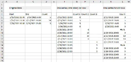
You can rearrange your data into three separate blocks as shown below. Select the first block, and insert an XY Scatter chart. Select and copy the second block, select the chart, and use Paste Special to add the data as new series, with series names in first row and X values in first column. Repeat with third block. With a little formatting, it looks like the chart below.

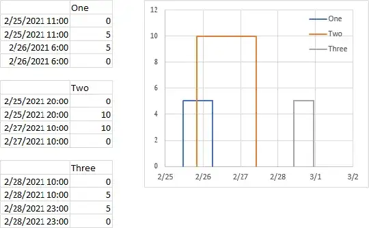
Or you can rearrange your data into one block with some blank rows between sections. Create an XY Scatter chart, and do the formatting.

You can download my workbook from here: Bar With Start and End Time.xlsx

EDIT: VBA approach to arrange data.

I have written a VBA routine that starts with data like the first block in the screenshot below, does minimal validation (is it three columns, is there a header row), asks the user which output is desired (one series for each row or one series for all rows combined), asks the user where to put the output, then produces the appropriate output. The output cells link to the input cells, so if the user changes a value in the input range, the output value will reflect the change.

It's minimally documented, feel free to ask questions.

The user first selects the input range (or one cell in the input range) and runs the code.

After running the code, the user needs only select the output range (or one cell in the output range), and insert an XY Scatter Chart with Lines and no Markers.

Here is the VBA procedure:

Sub Reformat_StartTimeCount_OneSeries()
  If TypeName(Selection) <> "Range" Then
    MsgBox "Select a range of data and try again.", vbExclamation, "No Data Selected"
    GoTo ExitSub
  End If
' input range: three columns (start, end, count), one row box, maybe header row
  Dim InputRange As Range
  Set InputRange = Selection
  If InputRange.Cells.Count = 1 Then
    Set InputRange = InputRange.CurrentRegion
  End If
  If InputRange.Columns.Count <> 3 Then
    MsgBox "Select a three-column range of data and try again.", vbExclamation, "No Data Selected"
    GoTo ExitSub
  End If
' one or multiple colors
  Dim Question As String
  Question = "Do you want one series (one line color) for each row of data?"
  Question = Question & vbNewLine & vbNewLine & "(Yes for multiple colors, No for one color)"
  Dim Answer As VbMsgBoxResult
  Answer = MsgBox(Question, vbQuestion + vbYesNo, "How Many Lines")
  If Answer = vbYes Then
    Dim MultipleSeries As Long
    MultipleSeries = 1
  End If
' ignore header row
  If Not IsNumeric(InputRange.Cells(1, 3)) Then
    Dim HasHeaderRow As Boolean
    HasHeaderRow = True
    With InputRange
      Set InputRange = .Offset(1).Resize(.Rows.Count - 1)
    End With
  End If
' how many rows?
  Dim RowCount As Long
  RowCount = InputRange.Rows.Count
' build array of formulas
  Dim OutputArray As Variant
  ReDim OutputArray(1 To RowCount * (5 - MultipleSeries) + MultipleSeries, 1 To 2 + MultipleSeries * (RowCount - 1))
Dim RowIndex As Long
  For RowIndex = 1 To RowCount
    Dim RowBase As Long, ColumnBase As Long
    RowBase = (RowIndex - 1) * (5 - MultipleSeries)
    ColumnBase = 2 + MultipleSeries * (RowIndex - 1)
    If MultipleSeries Then
      If HasHeaderRow Then
        OutputArray(1, ColumnBase) = "=" & InputRange.Cells(0, 3).Address(False, False) & "&"" " & RowIndex & """"
      Else
        OutputArray(1, ColumnBase) = "Count " & RowIndex
      End If
    Else
      If RowIndex = 1 Then
        If HasHeaderRow Then
          OutputArray(RowBase + 1, 2) = "=" & InputRange.Cells(0, 3).Address(False, False)
        Else
          OutputArray(RowBase + 1, 2) = "Count"
        End If
      Else
        OutputArray(RowBase + 1, 2) = "#n/a"
      End If
    End If
    OutputArray(RowBase + 2, 1) = "=" & InputRange.Cells(RowIndex, 1).Address(False, False)
    OutputArray(RowBase + 3, 1) = "=" & InputRange.Cells(RowIndex, 1).Address(False, False)
    OutputArray(RowBase + 4, 1) = "=" & InputRange.Cells(RowIndex, 2).Address(False, False)
    OutputArray(RowBase + 5, 1) = "=" & InputRange.Cells(RowIndex, 2).Address(False, False)
    OutputArray(RowBase + 2, ColumnBase) = 0
    OutputArray(RowBase + 3, ColumnBase) = "=" & InputRange.Cells(RowIndex, 3).Address(False, False)
    OutputArray(RowBase + 4, ColumnBase) = "=" & InputRange.Cells(RowIndex, 3).Address(False, False)
    OutputArray(RowBase + 5, ColumnBase) = 0
  Next
' output formulas
  Dim OutputRange As Range
  On Error Resume Next
  Set OutputRange = Application.InputBox("Select the top left cell of the output range.", "Select Output Range", , , , , , 8)
  On Error GoTo 0
  If OutputRange Is Nothing Then GoTo ExitSub
With OutputRange.Resize(RowCount * (5 - MultipleSeries) + MultipleSeries, 2 + MultipleSeries * (RowCount - 1))
    .Value2 = OutputArray
    .EntireColumn.AutoFit
  End With
ExitSub:
End Sub

I have uploaded a new workbook, which contains both parts of the answer. Download it here: Bar With Start and End Time.xlsm

Creating Bar Chart with Start time and End time

1 Answers1