How do I arrange data with the similar values in one of the columns together in Excel?

Question

I have an Excel table with 4 columns - name of the company, website, area, and description. How do I group the companies from the same area (column 3 in my case) together?

For example, this is what I have (more than 200 rows - too much to sort manually):

Answer 1

If you have a header row, you can take advantage of Excel's built-in sorting and filtering. If you don't already have one, follow the instructions in section 1 below, otherwise skip to section 2.

1. Making a header row

Go to the very first cell in the spreadsheet, and locate the following button in your Home ribbon at the top of your window:

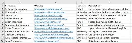
Click the down arrow and choose "Insert sheet rows". Then you can enter a header label for each column in the first row. Optionally you can make them bold, so they stand out from your data. You should end up with something that looks like this:

2. Sort and filter

Now, select your headers:

Then click the following button back in your Home ribbon (it should be near the right of your screen):

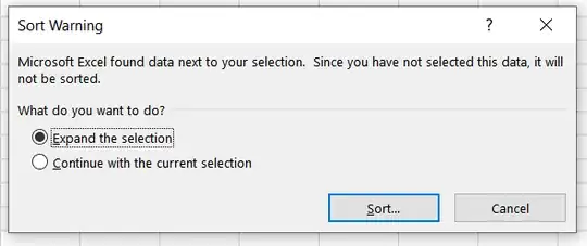
Select "Filter" from the drop-down menu. You will see dropdown boxes appear on your header cells, but let's ignore those for now. Click on the button again and choose "Custom Sort...". You will see a warning message:

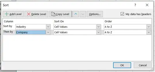
Make sure "Expand the selection" is selected and click "Sort...". This will take you to a window where you can specify how you want to sort your data. For your example, I would suggest the following:

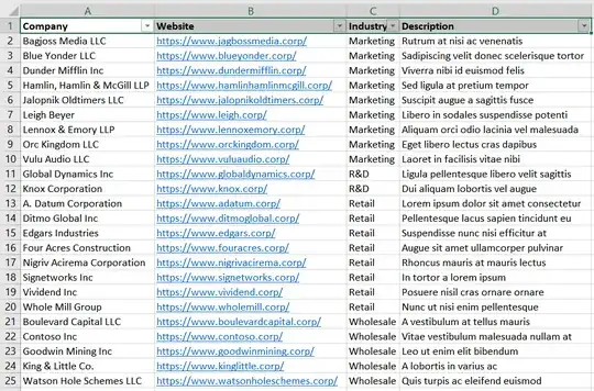
This groups all the industries together and then sorts companies alphabetically within that grouping. Here's the end result in my example spreadsheet:

3. Using filters

With those buttons we created earlier, you can also filter your data to show only one industy at a time:

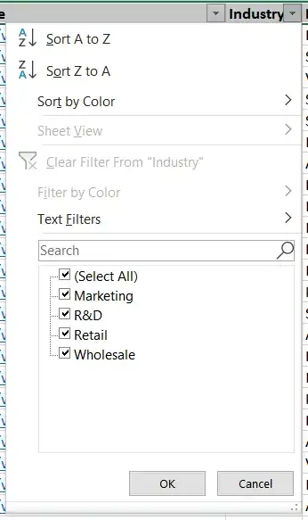
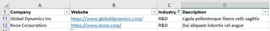
If you uncheck all the boxes except R&D and click OK, this is what you'll be left with:

To clear the filter, you can either use the dropdown menu from the column header, or you can clear multiple column filters at once using the Sort & Filter dropdown menu in the Home ribbon (which you used earlier).

4. Pivot tables

Another way Excel lets you group, sort, and filter data is using something called a Pivot Table. This is a very advanced feature and not really necessary for a fairly small data set like this, but I'd encourage you to watch some video tutorials if you're curious!