Why this apparent orthogonality in Excel's INDEX() syntax?

Question

TL;DR

In Excel 365:

1. Why doesn't a 0 in the second argument of INDEX(A1#,0,{1,3}) return all rows, when it does in each of INDEX(A1#,0,1) and INDEX(A1#,0,3)?
2. And is there a canonical way of getting it to do so?

DETAILS

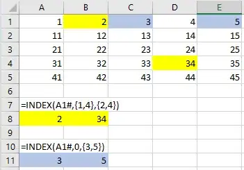
Assume I have a dynamic array rooted at A1. If I want the 1st column, all the rows, I can write:

=INDEX(A1#,0,1)

where the 0 in the second argument is the "all the rows" indicator. Similarly, if I want the 3rd column, I can write:

=INDEX(A1#,0,3)

And so if I want both the 1st and 3rd columns, I'd like to be able to write:

=INDEX(A1#,0,{1,3})

But that doesn't give what I expected. It does give the 1st and 3rd columns, but only the 1st row. That is, it gives exactly the same as:

=INDEX(A1#,1,{1,3})

To get what I want, I need to have that second argument mention every desired row. So, for example, what I'm often finding myself doing is this kind of thing:

=INDEX(A1#,SEQUENCE(ROWS(A1#)),{1,3})

That works, but it's a bit verbose.

Am I missing something? Is there a neater way of specifying "all the rows", in the way 0 does when asking for only one column?

And as a followup: can anyone explain why they might have built it like this? It seems to break orthogonality, but that might just be me.

P.S. I know there are entirely other ways of doing this kind of multi-non-contiguous column slice thing. For example:

= HSTACK(INDEX(A1#,0,1),INDEX(A1#,0,3))

But that's not much less verbose than the SEQUENCE() approach.

Answer 1

And is there a canonical way of getting it to do so?

As gns100 commented, in Excel365 you can use =choosecols(A1#,1,3).
Unfortunately no good solution in earlier versions.

Why doesn't a 0 in the second argument of INDEX(A1#,0,{1,3}) return all rows, when it does in each of INDEX(A1#,0,1) and INDEX(A1#,0,3)?

Having a look at output of =INDEX(A1#,{1,4},{2,4}) might help to understand the situation:

Instead of giving back intersection of (1st & 4th row) and (2nd & 4th) column, it gives values from coordinates 1,2 & 4,4; so when you provide two lists, it translates them to coordinates first.

As for why it only returns values from 1st row when you use 0, is probably due to how Excel converts 0 to a list in the background.