Excel heatmap with 2 color rules - possible? Using trunc?

Question

I have two tables showing the amount of Compound A and Compound B in the same samples. For example:

Compound A

	Sample 1	Sample 2
Condition x	0.5	0.01
Condition y	0.05	0

Compound B

	Sample 1	Sample 2
Condition x	0.03	0.01
Condition y	0.3	0.6

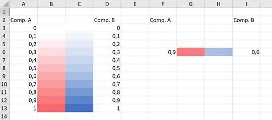
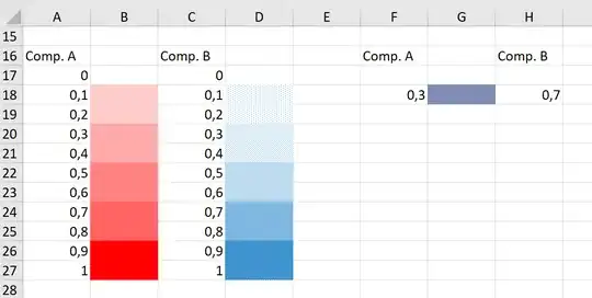
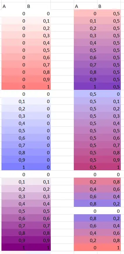
I would like to build a table / heatmap where I can see the information in both of the above tables combined in a visual way via Conditional Formatting. The idea would be to overlap two rules for coloring cells in conditional formatting (I don't know if this is possible). For example, if the maximum for A is marked in red, for B in blue and the minimum for both is white, then something with just A will look pink-red, something with just B will look blue-ish, and something with both A and B will appear in various shades of purple.

My initial idea was to first combine the information from both tables in a new table where, for instance, the information from Compound A would be encoded before the decimal point, and the information from Compound B, after the decimal. Like this:

Compound A*100 + Compound B

	Sample 1	Sample 2
Condition x	50.03	1.01
Condition y	5.3	0.6

Then I considered using TRUNC to get the values without the decimal (from there, I could easily get just the decimals). For example, for two color-formatting, I had formulas for:

Minimum:
=MIN(TRUNC($A$1:$B$2))

Maximum:
=MAX(TRUNC($A$1:$B$2))

However, this results in no colored cells. It works if I remove TRUNC, but that defeats my purpose.

I would appreciate if someone could have a look and tell me if what I am planning is possible, and if so, what am I doing wrong.

When trying to get information about the version, I get 'Microsoft Office LTSC Professional Plus 2021'.

score 1 · Accepted Answer · answered Oct 09 '23 at 21:12

You cannot use two color scales in the same cell. There are two reasons for that: first – cell must contain value which is the base of formatting, second – colors cannot be mixed or added if they relate to the same object - in this case cell interior fill.
So if you want to use color scales – you can use two neighboring cells.

Another possibility is to use two different properties of the cell: interior fill and interior pattern with different colors. The cell may contain data for 1 value, which refers e.g. to compound B and interior color for compound A may be defined with a formula.
However in this case you should define separate rules for each shade of color. Generally it is quite a complicated task.

example workbook

score 0 · Answer 2 · answered Oct 10 '23 at 12:56

You can do this through VBA. Here is an example; you may want to tweak the colors to suit your needs:

Function myColour(compoundA As Double, compoundB As Double)
      ' takes two concentrations (0-1) and converts to RGB
    Dim myRed, myGreen, myBlue As Integer
    If (compoundA >= 0 And compoundB >= 0 And compoundA <= 1 And compoundB <= 1) Then
        myGreen = 255 - compoundA * 127 - compoundB * 127
        myRed = 255 - compoundA * 127
        myBlue = 255 - compoundB * 127
    Else ' no valid values, make it grey
        myGreen = 127
        myRed = 127
        myBlue = 127
    End If
    myColour = RGB(myRed, myGreen, myBlue)
End Function
Sub colourMe()
        ' select a range of two columns (compound A, compound B) before running this macro
    Dim rng As Range
    For Each rng In Selection.Rows
        rng.Interior.Color = myColour(rng.Cells(1).Value, rng.Cells(2).Value)
    Next rng
End Sub

Here is the result, for a couple of combinations:

Excel heatmap with 2 color rules - possible? Using trunc?

2 Answers2