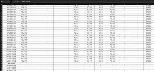
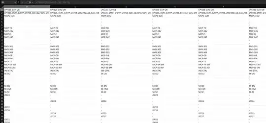
I have a large spreadsheet (679 rows x 243 columns) consisting of a series of product SKUs in the first column, and each subsequent column represents an accessory. Every SKU to which the given accessory is applicable has the accessory part number populated. Because not every accessory is applicable to every SKU, a significant number of cells are populated by a dash (signifying "N/A").

I need to reorder this data in two columns: the first column to contain the product SKU, and the second column to contain the applicable accessory part numbers (each on its own row). The first column will repeat the product SKU in as many rows as necessary until all applicable accessories for that SKU have been populated. Subsequent SKUs will be populated similarly on subsequent rows. No dashes are to appear in the final accessories column.

How can I accomplish this automatically? Multiple steps are fine, I'm just trying to avoid manually copying/pasting/deleting data by hand.
TRANSPOSE puts the accessory numbers (and dashes) in columns as desired, but the SKU is put once as a column header rather than repeated in a parallel column. If I could insert a new column to the left of each existing column and populate the existing column header in every row that has data, I could then use VSTACK to place all the data in two columns. Then I could delete the rows with dashes with a column filter.
