Summarizing data from an Excel table that has sub headers and sub totals

Question

I have a table in Excel that has some rows that define a subsection of the data. These subsections have a subtotal in them. I'd like to do a summary of the data from this table (essentially a pivot table), but I want to do it using the subsection headers. Since this is all in the same columns, I don't know how to go about doing this. This is something that I want to add to many files that I receive, so I don't want to have to do formatting of the excel file. I'm hoping for a formula I can just cut and paste to get me what I want. Not sure if this is even feasible.

That data looks somewhat like this:

Description	Quantity	Rate	Amount
Department 1
Item 1	10	$2	$20
Item 2	5	$3	$15
		Subtotal	$35
Department 2
Item 1	12	$2	$24
Item 2	6	$3	$18
		Subtotal	$42

What I would like to summarize would look like:

Department	Total Quantity	Total Amount
Department 1	15	$35
Department 2	18	$42

In reality, me data example is a bit more complicated than that, but if I could do that, then I could solve the more complex problem, I think.

Mayukh Bhattacharya · Answer 1 · 2024-11-01T21:29:25.270

There are many ways of accomplishing the desired output, here are few alternative ways which works based on ones Excel Version they are using(MS365 versions updated)

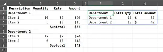
• Formula used in cell F2

=LET(
     a, A2:D9,
     b, SCAN(,IF(INDEX(a,,2)="",TAKE(a,,1),""),LAMBDA(x,y,IF(y="",x,y))),
     c, GROUPBY(b,CHOOSECOLS(a,2,4),SUM,,0,,b<>0),
     VSTACK({"Department","Total Qty","Total Amount"}, c))

This can also be accomplished using Power Query, available in Windows Excel 2010+ and Excel 365 (Windows or Mac)

To use Power Query follow the steps:

First convert the source ranges into a table and name it accordingly, for this example I have named it as Table1

Next, open a blank query from Data Tab --> Get & Transform Data --> Get Data --> From Other Sources --> Blank Query

The above lets the Power Query window opens, now from Home Tab --> Advanced Editor --> And paste the following M-Code by removing whatever you see, and press Done

let
    Source = Excel.CurrentWorkbook(){[Name="Table1"]}[Content],
    AddedCondition = Table.AddColumn(Source, "Dept", each if [Quantity] = null then [Description] else null),
    FillDown = Table.FillDown(AddedCondition,{"Dept"}),
    Filter = Table.SelectRows(FillDown, each [Description] <> null and [Description] <> ""),
    Answer = Table.Group(Filter, {"Dept"}, {{"Total Quantity#(tab)", each List.Sum([Quantity]), type nullable number}, {"Total Amount", each List.Sum([Amount]), type nullable number}})
in
    Answer

Lastly, to import it back to Excel --> Click on Close & Load or Close & Load To --> The first one which clicked shall create a New Sheet with the required output while the latter will prompt a window asking you where to place the result.

Also, if you are not interested in using these above, then also it can be achieved using Pivot Tables.

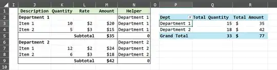
First, add a helper column after the amount column, and enter the following formula and fill down (note that you will need to change the cell range and references as per your data:

=IF(K2="",J2,N1)

Select any cell in the data and hit ALT+D+P it opens up the Pivot Table and PivotChart Wizard
Step One --> Don't press anything by default, it will selected Pivot Table, press only Next
Second Step --> Verify the wizard has selected the required range and hit Next
Third Step --> You can either select New Worksheet or Existing Worksheet with preferred cell references to place the pivot and hit Finish
From the Pivot Table Fields add the Helper in Rows Area while the Qty and Amt in the Values Area
Change the layout of the Pivot from the Design tab to Tabular Form and change the helper header to Dept or whatever suits you best. Other necessary formatting you can do as per your requitements. This will give you the exact output you needed.

score 0 · Answer 2 · answered Nov 02 '24 at 02:11

get the last data cell by looking up non-blank in column
XLOOKUP(TRUE, D:D <> "", D:D, , , -1)
get the row numbers for rows with department header and use it grouping
XLOOKUP(r, dept_rows, dept_rows, , -1, 2))
sum_col, LAMBDA(col, MAP(dept_rows,...

=LET(last, XLOOKUP(TRUE, D:D <> "", D:D, , , -1),
  data, A2:last, dept_col, A:A, qty, INDEX(data, , 2), amt, INDEX(data, , 4),
  note, "--- update values above to match data ---",
  dept_rows, FILTER(ROW(data), ISBLANK(amt)),
  dept_row, LAMBDA(r, XLOOKUP(r, dept_rows, dept_rows, , -1, 2)),
  sum_col, LAMBDA(col, MAP(dept_rows,
    LAMBDA(d, SUM(FILTER(col, ISNUMBER(qty) * dept_row(ROW(col)) = d))))),
  VSTACK(
    {"Department","Total Quantity","Total Amount"},
    HSTACK(CHOOSEROWS(dept_col, dept_rows), sum_col(qty), sum_col(amt))))

Summarizing data from an Excel table that has sub headers and sub totals

2 Answers2