I ran into this same issue myself recently, and while Google search got me to this question, I didn't feel that any of the existing answers really address it properly. But taking existing answers as a hint, I was able to do this in the following way:
Assume cell A1 contains the result of a calculation that gives a "negative time value". You can display a "sensible" time value (no ####) by entering the following in cell B1:
=IF(A1<0, TEXT(-A1, "-[H]:MM"), TEXT(A1, "+[H]:MM")
This turns the value into a string which you can format however you need - I chose to format with [H]:MM but you can use any valid Excel format. You do have to add the sign "manually".
Here is a screenshot of an application of this - where there is a cumulative sum of hours with occasional "payments" that can sometimes reduce the sum to a negative number. I expect that's quite a common thing, given some of the questions I have read on this topic.
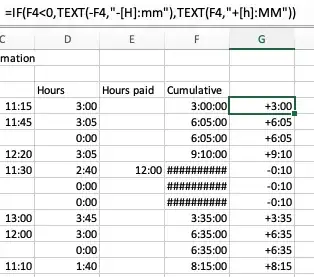
The only drawback of this method is that the time being displayed is in fact "text". If you need to manipulate the actual time result (including negative values) you should use the value, not the formatted version. You can do this by having a hidden column (if you want to keep your sheet "pretty") - this column can then be used for additional calculations, graphs etc. In the image below, column F has the "real" value while column G contains the "formatted" value.
You can even use conditional formatting with a formula rule to color these text fields "as though they were numbers"... but that was not the question.

![Screenshot of the cell format dialog in Excel. Within the Number tab we set a custom format for the cell to [mm] which displays the negative time difference in minutes.](https://i.sstatic.net/BCYSNl.png)