81

I use three columns. A, B and C. In column C I have a formula every row =A1*(1.6*B1) and then for the next row I have =A2*(1.6*B2) in C2.

How can I do so I don't have to type in the new formula in column C for every row?

I use it in both Google Docs SpreadSheet and OpenOffice SpreadSheet.

Jonas
  • 28,660

9 Answers9

93

Using the Mouse

  1. Click the cell whose formula you want to repeat
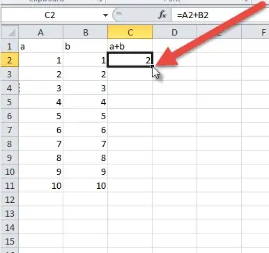
  2. A dark square "handle" will appear in the lower right corner

    Location of Drag box

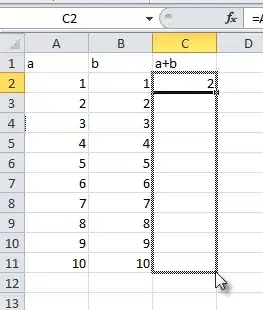
  3. Click and drag that handle, dragging down the column (or right across the row). You can also double click the handle to auto-fill.

    Dragging the box

  4. Stop at the last cell you wish to fill

Using the Keyboard

  1. Move the cursor to the cell whose formula you want to repeat
  2. Hold shift
  3. While holding, press down repeatedly to select the rest of the range of cells you want to fill
  4. When you reach the bottom, release shift then press CTRL + D (Use CTRL + R if you're filling to the right)(Using this method also preserves notes, unlike the mouse solution.)

In both cases what you're doing is called "filling." It is supported by every(?) spreadsheet program.

Geoff
  • 1,148
83

An even easier solution in Google Sheets would be to enter this formula in C1:

=ARRAYFORMULA(IF(A5:A,A5:A*(1.6*B5:B),""))

It automatically propagates to subsequent rows if a value is entered in column A, removing the need to copy it to each row. In fact, if you copied it to C2, it would be automatically overwritten by the continuation of the formula in C1.

The important part is the :A and :B, which specify you'd like to include these entire columns in your formula. This means you could apply the single cell formula =A5*(1.6*B5) to entire columns with:

=ARRAYFORMULA(A5:A*(1.6*B5:B)) 

Note that this yields bad results where A and B are missing values, so we wrap it in an IF() statement (see above) to show nothing when there are no values. You could also use IFERROR() to handle bad results.
Allison
  • 103
16

The suggested answers work well for small sheets but I had thousands of rows and using the mouse or the keyboard to select them was simply too time consuming.

The ARRAYFORMULA method works but it's complicated, forces me to rewrite formula style and consider possible errors).

The solution is so simple it can be done in 2 seconds:

  1. Write your new formula in the first CELL.
  2. click on the cell, press CTRL+C (copy the cell)
  3. click on the column header (for example A) to select the whole column
  4. CTRL+V -> paste the cell formula into the whole column
  5. profit
John
  • 396
  • 1
  • 4
  • 9
13

here is a another way, go ahead and delete all the formulas that are in there right now, then type in the formula in C1 having it correspond to A1 and B1 and hit enter.
so now the correct formula is just in C1,
now click the C1 box, a bounding box will appear, the bottom right corner of this bounding box has a dark square,
double click this square and the formula will 'fill down'
you will notice C2 corresponds to A2 and B2 and so on.
if this is what you need and i am understanding correctly

fightermagethief
  • 863
  • 4
  • 12
  • 26
7

I found all of these solutions very frustrating and confusing also.

I will warn you though, this will replace whatever is currently in the cells, but as it is a formula this should not be a problem.

For me it was simple.

  1. Click the cell whose formula you want to copy once (select it)
  2. Copy the cells contents (Ctrl+C on Windows, cmd+C on macOS)
  3. Hold Shift+Ctrl+Down (selecting all of the cells in that row)
  4. Now Paste the formula as you have all of the cells selected.

This will put the formula, updated with each cells on references.

phuclv
  • 30,396
  • 15
  • 136
  • 260
6

Very similar to ceoliphant's answer but a little more straightforward, simply add one formula to C1:

=ARRAYFORMULA(iferror(A:A*B:B*1.6))
skube
  • 249
5

After you write your forumla, you can double click the bottom, right corner of the selected cell with the blue box, to copy the data down the column down as long as a neighboring cell has data.

This saves a lot of time when you have a 7,000 row sheet you are working with.

enter image description here

3

P.S. I am working in OpenOffice, and now I see that it also works by simply copying the content of the cell and pasting it into the other ones. The formula is automatically adjusted to each row! (To avoid the automatic adjustment prefix the name of row number and column numbers with a $).

Mihai
  • 31
2

You could select the complete column C by selecting the header and paste the formula =A1*(1.6*B1) . it will apply to every row.

No need to select and drag to copy to every cell.