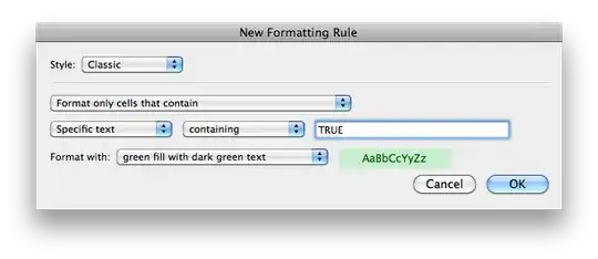
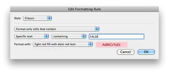
I have a range containing formulas that evaluate to TRUE or FALSE.
How would one apply conditional formatting to this range, so that TRUE cells are Green, and FALSE cells are RED?
I have a range containing formulas that evaluate to TRUE or FALSE.
How would one apply conditional formatting to this range, so that TRUE cells are Green, and FALSE cells are RED?


For Windows version. Microsoft 365 Excel (Version 2004(Build 12730.20270) *Note the version is not the year - this is the 365 version in year 2020
You need to create 2 rules (one for each colour) Go to
Home Tab -> Styles Group -> Conditional formatting -> Manage rules
*Alternatively just type Conditional formatting in the search bar at the top
New rule
Rule type -> Format only cells that contain
Cell Value -> Equal to -> {your value in this case True} =TRUE
And select the format, then okay
Now you should have 2 rules in your manage rules window
The usual Conditional Formatting rule of "Equal To" was not working for me when using "true"/"false"
I found that the "Text that Contains" option worked instead: