How to Label / Tag Items in a Spreadsheet

Question

I'm a novice at spreadsheets, so I hope you'll forgive me if I'm asking a super obvious question.

Is it possible to use tags in Excel/Google Spreadsheet? I'm creating a spreadsheet to log all the articles and books I'm reading. Say I'm reading "I, Claudius". I want to give it these tags: history, fiction, biography, disability, politics, drama. Then, if I want to display all the articles/books tagged with "politics", I can maybe search/display/pivot with that tag.

Maybe preferably, the tags should all be in one cell with each word separated by a comma. If each word were in a cell of its own, it would make the table really messy, I think.

I am open to other labelling solutions too.

Thanks!

Answer 1

As far as I know there are no built-in features that can parse and summarize comma-separated tags in Excel. You can, of course, create your own solution with worksheet functions and a little VBA. Here's a quick solution for doing this.

Step 1: Press Alt+F11 to open the VBA editor pane in Excel. Insert a new module and paste in this code for a custom function.

Public Function CCARRAY(rr As Variant, sep As String)
'rr is the range or array of values you want to concatenate.  sep is the delimiter.
Dim rra() As Variant
Dim out As String
Dim i As Integer

On Error GoTo EH
rra = rr
out = ""
i = 1

Do While i <= UBound(rra, 1)
    If rra(i, 1) <> False Then
        out = out & rra(i, 1) & sep
    End If
    i = i + 1
Loop
out = Left(out, Len(out) - Len(sep))
CCARRAY = out
Exit Function

EH:
rra = rr.Value
Resume Next

End Function

This function will allow you to create comma-separated lists to summarize the tag data you have.

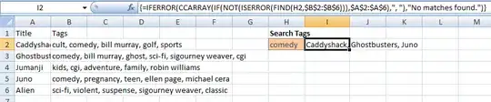
Step 2: In a worksheet, enter in a cell (H2 in the example below) the tag you want to search for. In the cell to the right, enter the following formula by pressing Ctrl+Shift+Enter.

=IFERROR(CCARRAY(IF(NOT(ISERROR(FIND(H2,$B$2:$B$6))),$A$2:$A$6),", "),"No matches found.")

By pressing Ctrl+Shift+Enter, you are entering the formula as an array formula. It will appear surrounded by {...} in the formula bar. Note that in the formula $B$2:$B$6 is the range that holds all the tags for the items listed in $A$2:$A$6.

EDIT:
If you don't mind your matches being listed in a column instead of in a list in one cell, you can return matches for tags using only worksheet functions.

Where your titles are in Column A, the tags are in Column B, and the tag you are searching for is in H2, you can use the following array formula in I2 and fill down as far as you need:

=IFERROR(INDEX($A$1:$A$6,SMALL(IF(NOT(ISERROR(FIND($H$2,$B$1:$B$6))),ROW($B$1:$B$6),2000000),ROW()-1)),"")

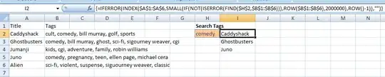
The formula works by first forming an array of numbers based on whether the tags in each row contains the search term. If a match is found, the row number is stored in the array. If it is not found, 2000000 is stored in the array. Next, the SMALL(<array>,ROW()-1) part of the formula returns the ROW()-1th smallest value from the array. Next, this value is passed as an index argument to the INDEX() function, where the value at that index in the array of titles is returned. If a number greater than the number of rows in the title array is passed to INDEX() as an argument, an error is returned. Since 2000000 is passed as the argument when no matches are found, an error is returned. The IFERROR() function then returns "" in this case.

It is important to grasp how ROW() is being used in this formula. If you want to display your list of results starting in a different row, you will need to adjust the second argument of the SMALL() function so that it returns the first smallest value from the array. E.g., if your list of results starts in Row 1 instead of Row 2, you would use SMALL(...,ROW()) instead of SMALL(...,ROW()-1).

Also, if your list of titles and tags does not start in Row 1, you will need to adjust the formula as well. The second argument of the IF() function must be adjusted so that a match in the first row of your data returns 1. E.g., if your list of titles starts in Row 2 instead of Row 1, you will need the formula to include IF(...,ROW($A$2:$A$7)-1,...) instead of IF(...,ROW($A$1:$A$6),...).

Answer 2

Another idea:

Use the inbuilt filter functionality. Filter by the Tags column, then you can search for rows containing a given tag.

A row with the tag list: comedy,horror,romance

would show up when searching for any of those three tags.

Answer 3

While doing this programmatically works well in some cases I found a manual approach worked for me. Using columns for tags you can easily tag a row item by entering a 0 into the column. You then have one row and enter 1s in each of the tag columns for that row (you can colour this row). Then when you sort by one of the tags the 1s (blue) row acts as a separator. Between your filtered results (0s) and everything else (_).

This has a few advantages. 1. You don't have to type your tag each time. 2. You can easily cross reference to check if you have duplicate or similar items that can be reduced to one.

Answer 4

My non-VBA approach is to list out tags in one column (let's say column H), separating items with commas. From there, I use a combination of "Text to Columns" and "Remove Duplicates" to get my list of tags. I copy past this into the header row of my main sheet (in this case, beginning in column L. Then, in each cell below the individual tag headers, enter the following:

=IF((ISNUMBER(SEARCH(L$1,$H2)))=TRUE,1,0)

This gives the best of both worlds - the tag column (H) is easy for people to read; the individual tag columns (with their 0s and 1s) are easy for the computer to read. It's dynamic if you remain within the given set of tags; if not, you need to add your new tag to the header row, then copy your formulas over.

From there, Pivot-Tables are your friend.

Answer 5

It's not clear to me exactly how you want to use the tags. But in Google Sheets, you can use the SPLIT() function to split a string of tags (delimited by spaces, commas, or whatever you want) into several other cells, and I'm sure even Excel has a function that can search a cell for a tag.