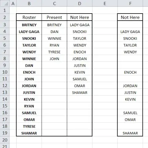
I've got two columns in Excel, "ROSTER" and "PRESENT", shown below:

Is there a formula to achieve the "NOT HERE" column? I tried using VLOOKUP() and https://superuser.com/a/289653/135912 to no avail =(
Any help would be appreciated!
Thanks!
I've got two columns in Excel, "ROSTER" and "PRESENT", shown below:
Is there a formula to achieve the "NOT HERE" column? I tried using VLOOKUP() and https://superuser.com/a/289653/135912 to no avail =(
Any help would be appreciated!
Thanks!
There is no built-in function that can singlehandedly do this task.
You can try this array formula in the "Not Here" column (MS Excel 2007+)
=IFERROR(INDEX(roster,SMALL(IF(COUNTIF(present,roster)=0,ROW()-1,""),ROW()-1),1),"")
Where (in my example)
roster is a Named Range that refers to $A$2:$A$21
present is a Named Range that refers to $B$2:$B$21
To enter the formula, select the cells in the Not Here column (in my case it's C2 down to C21), type the formula and then press Ctrl+Shift+Enter

This may be a bit overkill, but it works. Hopefully you don't mind having an intermediate 'Not Here' column with spaces, before arriving at the end result (Not Here 2).
Named ranges in use:
Array formula entered into range (D3:D19)...
{=IF(ISERROR(MATCH(Roster,Present,0)),Roster,"")}
Array formulae entered into cells (E3:E19)...
{=IFERROR(INDEX(NotHere,SMALL(IF(FREQUENCY(IF(NotHere<>"",MATCH(ROW(NotHere),ROW(NotHere)),""),MATCH(ROW(NotHere),ROW(NotHere)))>0,MATCH(ROW(NotHere),ROW(NotHere)),""),ROW(A1)),COLUMN(A1)),"")}
{=IFERROR(INDEX(NotHere,SMALL(IF(FREQUENCY(IF(NotHere<>"",MATCH(ROW(NotHere),ROW(NotHere)),""),MATCH(ROW(NotHere),ROW(NotHere)))>0,MATCH(ROW(NotHere),ROW(NotHere)),""),ROW(A2)),COLUMN(A2)),"")}
etc...
Though this looks a long-winded solution, it will work no matter where the table is placed within the worksheet. It also removes #num errors in Excel 2007, should you be using that version.