Excel - How to compare columns for equal values

Question

I have an Excel sheet which has two columns. Both columns have numbers. The first column contains more numbers than the second column. I want to find which all numbers in the second column are there in first column and which are not.

For example consider the following as an example:

Col A | Col B
1     |2
2     |5
3     |7
4     |10
5     |15
6     |
7     |
8     |
9     |
10    |
11    |
12    |
13    |
14    |
15    |

Answer 1

I would use a combination of IF and VLOOKUP. Assuming your data is in Col A and Col B, place the following formula in Col C

=IF(VLOOKUP(B2,A:A,1,FALSE), "Found", "Not Found")

Drag the formula down, and the results for your example would be as follows.

Answer 2

I'm sure there's a better way to do this, but my method involves a bit of a hack with NOT, ISERROR, and VLOOKUP.

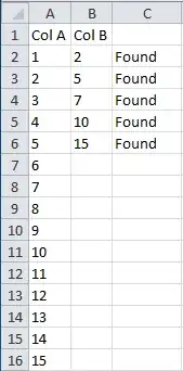
For checking the value in B2 against a list in column A, use the following:

=NOT(ISERROR(VLOOKUP(B2,A:A,1,FALSE)))

Step-by-step:

• VLOOKUP checks a value against a column of data, and returns data from a chosen cell in the same row where the lookup value was found.
  • B2 is the lookup value we're giving to VLOOKUP.
  • A:A is the range we want VLOOKUP to look in. You can use multi-column ranges if you want to pull data from a different column, but VLOOKUP will only search for the lookup value in the first (leftmost) column of the range.
  • 1 is the column we're telling VLOOKUP to pull data from. This is required by VLOOKUP, but really irrelevant to us since we're not actually using the data. This can be used to pull data from other columns in the matching row, so long as they are within the range specified in the preceding argument. VLOOKUP counts columns starting with 1 as the leftmost column in the range.
  • FALSE specifies an option for VLOOKUP that says we want an exact match. Otherwise, it can return inaccurate results for our needs here.
• ISERROR returns a boolean TRUE or FALSE to say whether or not processing the nested formula resulted in an error. So, we're not actually using VLOOKUP to get any data here - it's just being used to see if it can be run without an error with the given values.
• NOT reverses the boolean value provided by the nested formula.

VLOOKUP will try to find the value of B2 in column A. If it has a problem (if your formula and data are correct, this should only happen when B2 does not exist in A:A), it will throw an error. This will make the result of IFERROR to be TRUE. However, since our question is "Is the value there?" instead of "Is the value not there?", we use NOT to switch it to FALSE. Simlarly, if there's not an error processing VLOOKUP, ISERROR will return FALSE which will be changed to TRUE (i.e.: "No error, the value was found.") by NOT.

Note that the above formula will return a boolean TRUE/FALSE - not the "Found"/"Not Found" values you asked for. I do this because boolean output is easier to work with if further processing on the information is needed. For a simple example, compare =IF(B2,"I found it!","No luck, Chuck!") to =IF(B2="Found","I found it!","No luck, Chuck!"). If you really want the output to be "Found"/"Not Found" though, use this variant:

=IF(ISERROR(VLOOKUP(B2,A:A,1,FALSE)),"Not Found","Found")

Since we're specifying our own output terms there, we don't need to use NOT to mess with ISERROR's output but we do need to keep in mind that TRUE on an ISERROR means the value was not found - so, we put "Not Found" for value_if_true and "Found" for value_if_false.

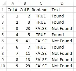
Here's a screenshot of both methods in action. The first formula in this answer was used for column C, the second is in column D.