Compare multiple columns for any two or more cells within the same row having the same content

Question

I need a formula to compare multiple columns for any two or more cells within the same row having the same content. If that is true, then display "TEXT A" (can be anything such as "TRUE"). If all of the values are different, display "TEXT B" or simply "FALSE".

I'm using an IF formula but it will be time-consuming if there are many columns to compare, so I need a better formula.

=IF((B2=C2);"YES";IF((B2=D2);"YES";IF((C2=D2);"YES";"ALL DIFFERENT")))

The same goes with similar function with OR (resulted in true or false)

=AND(($C2<>$D2);($C2<>$E2);($D2<>$E2))

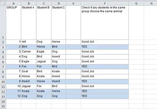
Below is a screenshot of the worksheet, which is just an example. My actual work has more than 4 columns.

The highlighted rows are the ones where there are two or more cells containing the same text (Group 2 should also be highlighted), hence those should display the "TEXT A" message.

View my Spreadsheet online

Answer 1

This VBa does it (how to add VBa). I have provided a few options so you can scale it in the future, check out the first 12 lines or so where you can type in the various 'answers' . You can choose which is the starting row and ending row, where the results will be displayed and what words to show if there is a text match or not! Please note, the highlighting is due to the Excel Doc you provided, and nothing to do with the code.

Before running a VBa script, take a back up of the file - there is usually no undo option!

Sub DoTheThing()

'Answer these questions or ye walk the plank

Dim row As Integer
row = 2

Dim firstColumn As String
firstColumn = "B"

Dim lastColumn As String
lastColumn = "D"

Dim resultsColumn As String
resultsColumn = "G"

Dim isFoundText As String
isFoundText = "YES"

Dim isNotFoundText As String
isNotFoundText = "Good Job"

'***Below be for the cap'ains eyes only.

Do While Range("A" & row).Value <> ""

    Dim startChar As Integer
    startChar = Asc(firstColumn)

    Dim endChar As Integer
    endChar = Asc(lastColumn)

    Dim i As Integer

    Dim hasMatch As Boolean
    hasMatch = False

    For i = startChar To endChar

    If Range(Chr(i) & row).Value = Range(Chr(i + 1) & row).Value Then

        hasMatch = True

    End If

    If Range(Chr(startChar) & row).Value = Range(Chr(i + 1) & row).Value Then

        hasMatch = True

    End If

    Next i

    If (hasMatch) Then
        Range(resultsColumn & row).Value = isFoundText
    Else
        Range(resultsColumn & row).Value = isNotFoundText
    End If

row = row + 1


Loop

End Sub

I wrote the results to Col G (to keep your original as is)

After the vba is run

Answer 2

For cell F2:

=IF(SUMPRODUCT(--(FREQUENCY(MATCH(B2:D2,B2:D2,0),COLUMN(B2:D2)-COLUMN(B2)+1)>0))=3,TRUE,FALSE)

This will give you True whenever there are three distinct values in those three columns.

Adapted from a site which includes more explanation and an option for dealing with blanks: https://exceljet.net/formula/count-unique-text-values-in-a-range

The same site touches on countifs and the potential for performance problems with large sets of data: https://exceljet.net/formula/count-unique-values-in-a-range-with-countif

Answer 3

Two-step solution without array formulas:

Step 1: For each column calculate number of occurences. If it's greater than 1 then put 1, otherwise empty string. Formula for cell D2 on the screenshot:

=IF(COUNTIF($A2:$C2,A2)>1,1,"")

This formula can be dragged (or double-clicked) by the bottom right corner to cover all rows, then the whole selected row D can be dragged by the bottom right corner to cover all columns.

Step 2: For each row check if there was any "1"

Formula for cell G2 on the screenshot:

=IF(SUM($D2:$F2)>0,"YES","Good Job")

This formula can be dragged (or double-clicked) by the bottom right corner to cover all rows.

In order to make it nicer, you might consider moving the intermediate calculations to another sheet.

Answer 4

Formula for D2 on the screenshot:

=IF(MAX(COUNTIF($A2:$C2, $A2:$C2))>1,"YES","Good job")

Enter it as an array formula by pressing Ctrl+Shift+Enter when editing the formula. After that it can be dragged (or double-clicked) by the bottom right corner to cover all rows.

Answer 5

There is a straightforward way to do this with formulas. Let me point out that the example shows cases that only involve matches that include the first column. Any formula should be tested against an example that contains random matches.

I'll explain this in two parts since the number of columns can vary. The first part is an expression that you build for the required number of columns. I've added a column of data to illustrate the formula better, and included some cases with random matches:

The expression for four columns of data looks like this (shown for row 2, the first data row):

    COUNTIF(C2:E2,B2)+COUNTIF(D2:E2,C2)+(D2=E2)

If N is the number of data columns, the formula contains N-1 terms. The first term counts how many columns have values that equal the first. The second counts how many of the remaining columns equal the second. And so on. They can all be COUNTIFs but I've used as simpler term for the last case. Instead of counting one column, I just test whether the next to last equals the last. A result of True is recognized as a value of 1, False as a value of 0. If all of the values are unique, this expression will equal 0. Otherwise, it will be a higher number. The expression goes inside an IF test:

    =IF(<expression>=0,"Unique Message","Match Message")

So for four data columns, the formula would be:

    =IF(COUNTIF(C2:E2,B2)+COUNTIF(D2:E2,C2)+(D2=E2)=0,"Unique Message","Match Message")

The result looks like this:

Answer 6

I would use the Power Query Add-In for this. It has a Group command with a Count Distinct function that can figure this out across any combination of rows and/or columns.

I've built a prototype which you can view or download - its "Power Query demo - compare multiple columns for unique values.xlsx" in my One Drive:

https://onedrive.live.com/redir?resid=4FA287BBC10EC562%21398

Note you can keep adding columns and/or rows to the Input sheet, then just hit Refresh All from the Data ribbon to reprocess the Power Queries.

90% of this was built just clicking around in the Power Query ribbon. The only exception was the simple "if" statement I wrote in the last step of the "Compare Multiple Columns" query. So there is far less code to maintain, compared to either a formula or VBA solution.

Answer 7

You can use this formula:

=IF(Cell Number > 2nd cell Number, result)