Using COUNTIF in Excel to count number of "Greater than" values in an array of values

Question

So here is my situation. I'm a principal creating a tracker for my teachers to use to track student growth on assessments. In the current tracker it is set up like this:

            % of            67%
            Students Met

**Student Name    Week 1 Goal:         Week 1 Actual:        Goal Met?:**
  Example A       23                    32                    Y
  Example B       45                    44                    N
  Example C       53                    55                    Y

I use a formula for the "Goal Met?" column to put a Y or N depending on if the Actual meets or exceeds the Goal column. Then, I use another formula to determine the % of students Met by doing a COUNTIF of "Y"s in the Goal Met column, dividing it by a COUNTA of that column, and multiplying by 100.

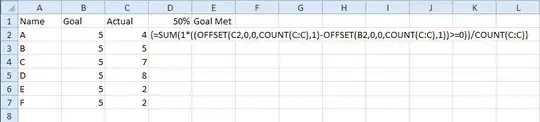
What I'm wondering is... this is very cumbersome to use for teachers, and the more columns and formulas I put, the greater the risk of teachers typing in the wrong place and messing up the formulas... is there any way I can just do a COUNTIF of the Array of the Weekly Goal and Weekly Actual columns, and count only the rows where the Actual is >= the Goal? Like is there a way to do COUNTIF(E5:F17,F>=E) and put some sort of symbol as a variable by the E and F in the criteria so that it goes row by row and compares the values, then counts the ones where the F value is greater than the E value?

Any suggestions would be great because then I can eliminate the "Goal Met" column (which they invariably type in and I have to go back and fix weekly). It gets annoying have to protect every 3rd column on a massive tracker!

Thanks so much for any advice!

Brendan

Answer 1

You should always password protect your cells that you do not want changed.

To answer you question you will need to enter an array formula. Type the following in assuming your column names starts on A3 and then hit Ctrl+Shift+Enter.

=SUM(IF(C4:C6>=B4:B6,1,0))/COUNT(C4:C6)

If you did it correctly curly brackets will appear around the whole formula.

={SUM(IF(C4:C6>=B4:B6,1,0))/COUNT(C4:C6)}

Answer 2

My Solution

The following array formula, with cell references adjusted appropriately, should do what you're looking for:

=SUM(1*((OFFSET(C2,0,0,COUNT(C:C),1)-OFFSET(B2,0,0,COUNT(C:C),1))>=0))/COUNT(C:C)

Example:

Set the C2 reference in the first OFFSET to the top cell of the 'Actual' data (F5 in your example), the B2 reference in the second OFFSET to the top cell of the 'Goal' data (E5 in yours), and set all of the C:C references to the column containing one or the other of the 'Actual' or 'Goal' data (E:E or F:F in yours). Be sure that the only cells with numerical data in the column you choose to replace the C:C references are those cells with 'Actual' or 'Goal' values in them, otherwise the formula will either return an inaccurate result, or will fail entirely.

To enter the formula as an array formula, type it in appropriately and then press Ctrl-Shift-Enter, instead of just Enter. (See here for more information on array formulas, or just search online for "excel array formula".) Any time you make a change to the formula, you will always have to enter it with Ctrl-Shift-Enter in order for it to behave properly.

How It Works

• Each COUNT retrieves the number of rows of data present.
• The two OFFSET calls retrieve the two arrays of interest, the 'Actual' and 'Goal' scores. In each call:
  • The first argument marks the top-left cell of the array;
  • The second and third arguments are the row and column offsets, respectively (both zero here);
  • The fourth argument indicates the number of rows to include in the array; and
  • The fifth argument indicates the number of columns to include.
• Since this is an array formula, subtracting the 'Actual' and 'Goal' arrays returns an array of the same size, but containing the element-wise difference between them.
• The >=0 comparison converts the array of differences into an array of TRUE/FALSE values indicating whether or not the goal was met.
• The 1* is there to convert the Boolean TRUE and FALSE values to numerical 1 and 0, to then be counted up by the SUM function.
  • In Excel, TRUE and FALSE implicitly carry the numerical values of one and zero.
  • BUT, if you try to pass a range or array containing TRUE/FALSE values to a function like SUM, it will ignore TRUE values and return zero.
  • SO, multiplying the whole TRUE/FALSE array by 1 is a way to trick Excel into interpreting the array in a useful way.
• The SUM divided by the COUNT is then the desired fraction of students meeting the goals set.

EDIT: Per wbeard52's answer, it should be possible in Excel 2010 or later to replace the 1*... hack with an IF structure. In older versions of Excel, IF mishandled array inputs.

Answer 3

Another couple of array formula options, so you need to press Ctrl+Shift+Enter to commit them.

To find the number of goals met:

=SUM(--(C4:C6>B4:B6))

To find the percentage of goals met:

=SUM(--(C4:C6>B4:B6))/count(C4:C6)

You can use them independently. Remember to enter them as array formulas by pressing Ctrl+Shift+Enter.

Answer 4

Another "array formula" approach is like this:

=AVERAGE(IF(E5:E17<>"",IF(F5:F17>=E5:E17,1,0)))

confirmed with CTRL+SHIFT+ENTER

That gives you an actual % like 0.5 - if you want 50 multiply by 100