0

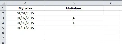
I have a spreadsheet that in column A lists dates. Column B may or may not have data in each cell.

The question I have is when I grab the last cell with data in column B, how can I also grab the corresponding data in column A?

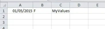
On a separate sheet, I wish to have 3 cells with data:

Cell 1 = the data in the last cell containing data in column B

Cell 2 = the corresponding date in column A

Cell 3 = the header of column B (the header will be different every time)

I’m using =LOOKUP(9.99E+307,B:B) to get the last cell with data in column B

I'll then repeat for the last cell with data in columns C, D, etc…

Dave
  • 25,513
Eric
  • 1

4 Answers4

2

So this looks up the value of the last non-blank

=LOOKUP(9.99E+307,B:B)

So then, this would lookup the row of the last non-blank

=MATCH(9E+99+307,B:B,1)

If you want to know what's next to it, you can use indirect -

=INDIRECT("A"&MATCH(9E+99+307,B:B,1))

Or you could use an index/match (probably a better choice)

=INDEX(A:B,MATCH(9E+307,B:B,1),1)
Raystafarian
  • 21,963
  • 12
  • 64
  • 91
0

With VBa, take a copy of the file first (there is no option to undo)

Try this

Option Explicit
Sub DoTheThingy()

Dim row As Integer
row = 2                     'start at 2 because we have headers

Dim myDate As String
Dim myValue As String

Do While (Worksheets("Sheet1").Range("A" & row).Value <> "")

    If Worksheets("Sheet1").Range("B" & row).Value <> "" Then
        myDate = Worksheets("Sheet1").Range("A" & row).Value
        myValue = Worksheets("Sheet1").Range("B" & row).Value
    End If

    row = row + 1
Loop

Worksheets("Sheet2").Range("A1").Value = myDate
Worksheets("Sheet2").Range("B1").Value = myValue
Worksheets("Sheet2").Range("C1").Value = Worksheets("Sheet1").Range("B1").Value
End Sub

Also see How do I add VBA in MS Office?

Worksheet 1:

enter image description here

Worksheet 2 after I run the macro

enter image description here

Dave
  • 25,513
0

If you are using LOOKUP like this to get the last value in column B

=LOOKUP(9.99E+307,B:B)

....then you can simply add another column as 3rd argument to return the corresponding cell from that column, i.e.

=LOOKUP(9.99E+307,B:B,A:A)

barry houdini
  • 11,212
0

The above are very creative solutions, but you don't really need to do anything fancy. Match supports the "*" syntax. So =INDEX(A:A,MATCH("*",B:B,-1)) will get you there:)

Pillgram
  • 101