94

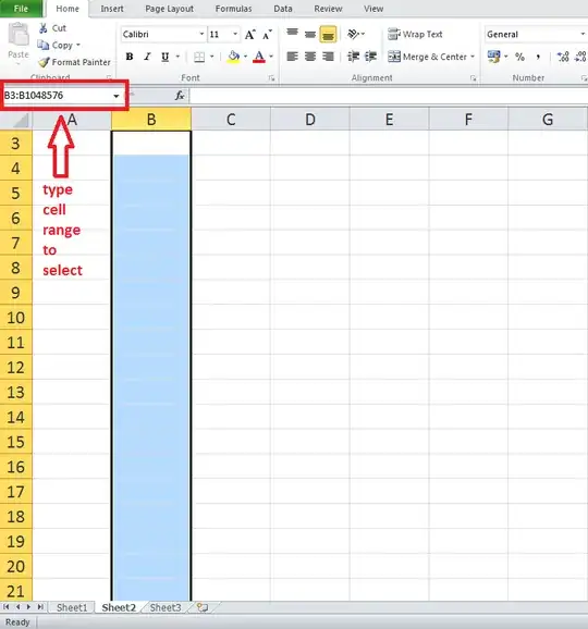
I know I can select all cells in a particular column by clicking on column header descriptor (ie. A or AB). But is it possible to then exclude a few cells out of it, like my data table headings?

Example

I would like to select data cells of a particular column to set Data Validation (that would eventually display a drop down of list values defined in a named range). But I don't want my data header cells to be included in this selection (so they won't have these drop downs displayed nor will they be validated). What if I later decide to change validation settings of these cells?

How can I selection my column then?

A sidenote

I know I can set data validation on the whole column and then select only those cells that I want to exclude and clear their data validation. What I would like to know is is ti possible to do the correct selection in the first step to avoid this second one.

I tried clicking on the column descriptor to select the whole column and then CTRL-click those cells I don't want to include in my selection, but it didn't work as expected.

Robotnik
  • 2,645

14 Answers14

94

Click on the first cell you want to be selected and then press Ctrl + Shift + to select a block of non-blank cells, or a block of blank cells (including the first non-blank cell below it), downwards.  Press again to extend the selection through further blocks.

This may cause the top of the worksheet to scroll off the screen.  Press Ctrl+Backspace to scroll back up quickly.

27

Universal

=SUM(A2:INDEX(A:A, ROWS(A:A)))

or

=SUM(A:A) – A1

Both will return summary for "column A", except for header in A1

BBK
  • 421
14

You can simply use the Name box, to the left of the Formula bar, and type the cell range you want selected. Once selected, you can also name this range so that you can use it's name as a reference in formulas and functions.


enter image description here

tzvi
  • 105
Peachy
  • 668
12

You can type F5 to bring up the name box. Then type B3:B65536 and click OK. 65536 for Excel 2003 and earlier, 1048576 for 2007 and 2010.

dkusleika
  • 1,846
8

If you wanted to exclude Header which I assume to be at row one, you can do this:

A2:A

For exmaple:

=SUM(A2:A)

which will include A2 and also everything after that in Column A.

Hope this answer help you.

Edit: I did this in Google sheets, and it doesn't work in Excel.

Dave M
  • 13,250
2

You can use the Ctrl Shift function and instead of using the to scroll through to the end you can just hit End and then one time and you will be at the end of the sheet instead of holding the forever ever.

You can also use the F5 function as well by hitting Ctrl+G then typing in whichever cell number your range starts in, ex: B5. It will take you to that cell. Once highlighted hit Ctrl+G again and type in any cell number in the range you want selected, ex: B7024 and BEFORE you hit Enter, hold down Shift and that exact range will be selected.

Or you can just exclude headers when doing data validation. Also, to select all cells if you go into A1 and hit Ctrl A once. It will select cells with data only, this is good to avoid blanks.

2

If you have column A of cells containing text, you can use the following to generate an array of all cells in colA excluding cell A1

=SUBSTITUTE(A:A, A1, "")

You can chain more SUBSTITUTE calls together if you need to exclude more cells. This is probably fine for a few excluded cells, but if it is any more complex you should probably use OFFSET.

1

Mario's answer up top (which was chosen) works, but I feel it is lacking since you are forced to go all the way to the bottom of the sheet - you then have to use another shortcut to center the screen back at the top of the sheet. Here is my solution (only tested in Excel 2013):

I tried clicking on the column descriptor to select the whole column and then CTRL-click those cells I don't want to include in my selection, but it didn't work as expected.

After clicking on the column descriptor and highlighting the entire column, hold down Shift and then press Tab, ,

The time between the Press of the Tab and the press of the first needs to be short or you will start tabbing from the bottom of the screen up, but not simultaneous or you then have to do more to get it to work.

If you then continue to hold the Shift button down you can now start removing cells from your list of highlighted cells from the top down by using .

santanaG
  • 111
1

Some of the answers here are good and some are wrong... If you want a more complex, but more flexible answer, here is my solution.

For example, to start from the 3rd row of the column C, you can use this

=SUM(OFFSET(C3,0,0,LOOKUP(2,1/(NOT(ISBLANK(C:C))),ROW(C:C))))

Where C3 is the first cell to be counted and both C:C from the last part are referring to the column you want to specify. The first 0 is if you want to shift the first (starting) cell down to another row and the second 0 is to shift the starting cell to another column. For example, if you still want to go for C3, but you want a more general example, you can use this (starting cell A1 + 2 rows + 2 columns = C3):

=SUM(OFFSET(A1,2,2,LOOKUP(2,1/(NOT(ISBLANK(C:C))),ROW(C:C))))

Success!...

0

An alternative method of selecting an entire column with the exception of the top cell is to use OFFSET to shift the range down by one cell. However, it is essential to prevent the range of the formula from overrunning the bounds of the sheet. Fortunately, OFFSET includes the facility to specify not only the shift but also the length of the range:

use OFFSET(A:A,1,0,COUNTA(A:A)-1)

e.g. SUM(OFFSET(A:A,1,0,COUNTA(A:A)-1))

Of course, this approach will also work for skipping more than one row at the top:

e.g. SUM(OFFSET(A:A,3,0,COUNTA(A:A)-3))

0

Write a VBA script that can be (de)activated with a shortcut.

Details of the VBA script:

  • The VBA script understands when a full column is selected and adds the last small step of taking away the x first cells.

  • Or the VBA script assigns names to the needed addresses of all filled columns, so that the mere column letter in the name field will select what you need, see @Peachy, or you just build the address automatically when you click on the column and afterwards press a key.

  • You might also be able to adjust the VBA script to mark everything below the frozen window line.

  • There are surely a lot more options using answers from here in VBA scripts.

questionto42
  • 2,691
0

Currently, if you are trying to select a column for a formula, it is as simple as using the term A2:A, or something similar.

In general, this can be used to select one or more columns, excluding some header space at the top, by including one of the top corner cells, followed by a colon, then the column at the other end of the range (this would be the same column if you are only trying to select one). For example, if I wanted the average of column C, but didn't want to include the two header cells at the top, I'd use =AVERAGE(C3:C), because C3 is the top cell I want to select. If I wanted the sum of columns B-E from row 3 down, I'd use =SUM(B3:E).

I believe this is a rather recent change, hence why the older answers are more complicated, but it makes this much more convenient.

-1
  • Choose the header field that you want to exclude from Data Validation rule
  • From the Menu choose Data -> Data Validation -> Data Validation
  • Press "Clear All" button
  • Press OK button

Now your header field will not have the data validation that was applicable for the rest of the column fields

Zubair
  • 1
-2

Right-click and choose Hide on the rows you don't want to get selected and then select whole columns.

Osku
  • 1