1

I'm trying to more fully automate the calculation of values and summary data in a spreadsheet I keep about the results of matches in a pool league.

I have a table with lots of information about each match, with the relevant fields being: Date of Match, Winner, Winner Starting Handicap, Winner Ending Handicap, Loser, Loser Starting Handicap, Loser Ending Handicap, Match Start Time.

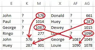
Handicaps are adjusted at the end of every match, and before the next one. It's a pain to find the most recent past record for a player (could have been a Winner or Loser) and copy his ending handicap from that record to the Starting Handicap (winner or loser) for the one I'm now entering.

I'd like a formula that would find the most recent record (highest date & start time in case he played twice in one day) where he was a winner or a loser, and then get the ending handicap (from the respective winner or loser).

Per teylyn's suggestion, here's a Dropbox link to the file. The relevant tab is Match Results: https://www.dropbox.com/s/1j9c6zsxjd3q4dt/Sample%20for%20Excel%20Question%20on%20Superuser.xlsx?dl=0

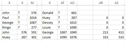
I added a blank column L to test things, comparing the results to what's in K to see if they were working, that's why it's there. Forgot to remove it when I put it in Dropbox.

1 Answers1

2

Problem Statement

A worksheet has names in Columns E and X.  For every row n, EnXn.  There are numbers in Column M corresponding to the names in Column E, and numbers in Column AG corresponding to the names in Column X.  For any row after the first (let’s say Row 42), we want to get values for K42 and AF42 from previous rows, if possible.

  • If E42 is “John”, find the most recent row that contains “John” (in Column E or X).  Call that row n.  If En = “John”, set K42 equal toMn.  If Xn = “John”, set K42 equal toAGn.
  • If X42 is “Scott”, find the most recent row that contains “Scott” (in Column E or X).  Call that row n.  If En = “Scott”, set AF42 equal toMn.  If Xn = “Scott”, set AF42 equal toAGn.


Solution

In the hopes of preserving some sanity, let’s use helper columns; let’s say AR and AS.  Assume that (as in the example file), data start in Row 2.  Enter

=MAX(($E$2:$E2=$E3)*(100*ROW($E$2:$E2)+COLUMN($M:$M)), ($X$2:$X2=$E3)*(100*ROW($X$2:$X2)+COLUMN($AG:$AG)))

into AR3 (skipping AR2).  End with Ctrl+Shift+Enter, to make it an array formula.  Likewise, set AS3 to

=MAX(($E$2:$E2=$X3)*(100*ROW($E$2:$E2)+COLUMN($M:$M)), ($X$2:$X2=$X3)*(100*ROW($X$2:$X2)+COLUMN($AG:$AG)))

as an array formula.  (This is the same as AR3 except the two occurrences of $E3 have been replaced with $X3.)

Set K3 to

=IF($AR3=0, "?", INDEX($A$1:$BG$999, INT($AR3/100), MOD($AR3,100)))

and AF3 to

=IF($AS3=0, "?", INDEX($A$1:$BG$999, INT($AS3/100), MOD($AS3,100)))

(not as array formulas).  These are the same except the three occurrences of $AR3 have been replaced with $AS3.

And, of course, drag/fill down.

The helper columns find the most recent previous occurrences of the names — ARn finds the most recent previous occurrence of En, and ASn finds the most recent previous occurrence of Xn — basically by finding the maximum, throughout the previous rows, of

(previous_value=this_value) * ROW())

i.e., the highest row number where the name is a match.  It then encodes the location where the name was found as

100*ROW() + COLUMN(data_we_want_to_copy)

Both formulas look in both Columns E and X, and return the encoded coordinates of the corresponding Columns M or AG cell.  Then the K and AF formulas simply decode the cell address and retrieve the value.


So AR6 is 213 because “John” (E6) was most recently seen on Row 2, and, since he was seen in E2 (rather than X2), we want to copy the value from Column 13 (Column M).