Excel: how to create multiple rows from one

Question

I have many rows in a document in which I need to insert a certain subset of rows with others. In particular, I need one row for each month considered. If I have the row starting with July and finishing with September, I need to replace that row with 3 rows, one for July, one for August and one for September.

How can I do it automatically?

Answer 1

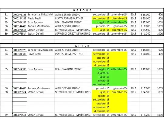
I assume that your data look like this:

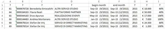
_{(1) I formatted columns E and F as mmm-yy (m/yyyy) to avoid language-based confusion.}
^{(2) There is a copyable version of the above in this answer’s source.}

on Sheet1, and that you want to copy it to Sheet2 with the extra rows added.  You can do that with three “helper columns” on Sheet2 — in the below steps, I use X, Y, and Z.  Here’s how to do it:

• Copy the column headings from Sheet1, row 1, to Sheet2, row 1.
• Enter =IF($Y2=0, INDEX(Sheet1!A:A, $X2), "") into Sheet2!A2 and drag/fill to the right to cover all your data (i.e., to column I).
• Copy Sheet1:A2:I2 and paste formats onto Sheet2:A2:I2.
• Change Sheet2!E2 (begin month) to
      =DATE(YEAR(INDEX(Sheet1!E:E, X2)), MONTH(INDEX(Sheet1!E:E, X2))+Y2, 1).
• Enter 2 in Sheet2!X2.  This designates the row on Sheet1 that this row (on Sheet2) will pull data from, so, for example, if your data actually begin in row 61 on Sheet1, enter 61 in Sheet2!X2.
• Enter 0 in Sheet2!Y2.
• Enter =INDEX(Sheet1!F:F, $X2) into Sheet2!Z2.  (If you want, format it as a date.)
• Select Sheet2!A2:Z2 and drag/fill down to row 3.
• Change Sheet2!X3 to =IF(E2<Z2, X2, X2+1).
• Change Sheet2!Y3 to =IF(E2<Z2, Y2+1, 0).
• Select Sheet2!A3:Z3 and drag/fill down as far as you need to get all your data.

It should look something like this:

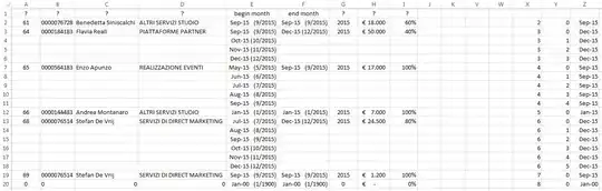
Notes:

• As stated in the instructions, Sheet2!Xn specifies the row on Sheet1 that row n (on Sheet2) will pull data from.
• Sheet2!Yn is a one-up number within a Sheet2!Xn value; i.e., within a Sheet1 row.  For example, since rows 3-6 on Sheet2 pull data fromSheet1 row 3, we have X3=X4=X5=X6=3, and Y3, Y4, Y5, Y6 = 0, 1, 2, 3.
• Column Z is just the “true” branch of the IF expression in column F; i.e., the end month for this group of rows.

Of course you can hide columns X, Y, and Z.  Or, if you want to do this just once and be done, you can copy and paste values.