3

I have three columns with values (A, B, C) as shown below. I would like a formula in column D that will return ALL the values from column B that are not listed in column A. Similarly, what formula should I write for column E that will return all values in column C that are not present in both columns A and B?

A   B   C   D   E
1   6   5       
5   7   7       
7   8   11      
10  9   12      
12  10  16      
    15  18      
        19      

In other words, I would like column D to give: 6, 8, 9, 15 and column E to give: 11, 16, 18, 19.
DavidPostill
  • 162,382
A.H.
  • 39

2 Answers2

2
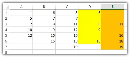
  • Column D: =IF(COUNTIF(A:A,B1)=0,B1,"") » Autofill down
  • Column E: =IF(COUNTIF(A:B,C1)=0,C1,"") » Autofill down

enter image description here

nixda
  • 27,634
1

It’s hard to do what you’re asking for all at once.  Things like this are best done using “helper columns” to hold intermediate results.  Here’s one approach:

  • Set F1 to =MAX(IF(B:B <> "", ROW(B:B)+3, 0)), typing Ctrl+Shift+Enter after you type the formula.
  • Set F2 to =INDEX(F:F, F1, 1).
  • Leave F3 blank.
  • Set F4 to =F3 & IF(AND(B1 <> "", COUNTIF($A:A, B1) = 0), B1 & ", ", "").  Drag/fill down to cover all your A/B data plus three rows.
  • Select Column F and drag/fill over to Column G.
  • Enter =LEFT(F2, LEN(F2)-2) in D1 and drag/fill over to E1.