Analytic Combinatorics/Singularity Analysis

This article explains how to estimate the coefficients of generating functions involving logarithms and roots.

You first may need to familiarise yourself with:

• Converting between Cartesian and polar coordinates
• Parameterising a curve

Theorem from Flajolet and Odlyzko^[1].

If:

${\displaystyle f(z)=(1-z)^{\alpha }\left({\frac {1}{z}}\log {\frac {1}{1-z}}\right)^{\gamma }\left({\frac {1}{z}}\log \left({\frac {1}{z}}\log {\frac {1}{1-z}}\right)\right)^{\delta }}$

where ${\displaystyle \alpha \notin \{0,1,2,\cdots \},\gamma ,\delta \notin \{1,2,\cdots \}}$ then:

${\displaystyle [z^{n}]f(z)\sim {\frac {n^{-\alpha -1}}{\Gamma (-\alpha )}}(\log n)^{\gamma }(\log \log n)^{\delta }\quad ({\text{as }}n\to \infty )}$

Theorem from Flajolet and Sedgewick^[2].

If ${\displaystyle f(z)}$ has a singularity at ${\displaystyle \zeta }$ and:

${\displaystyle f(z)\sim \left(1-{\frac {z}{\zeta }}\right)^{\alpha }\left({\frac {1}{\frac {z}{\zeta }}}\log {\frac {1}{1-{\frac {z}{\zeta }}}}\right)^{\gamma }\left({\frac {1}{\frac {z}{\zeta }}}\log \left({\frac {1}{\frac {z}{\zeta }}}\log {\frac {1}{1-{\frac {z}{\zeta }}}}\right)\right)^{\delta }\quad ({\text{as }}z\to \zeta )}$

where ${\displaystyle \alpha \notin \{0,1,2,\cdots \},\gamma ,\delta \notin \{1,2,\cdots \}}$ then:

${\displaystyle [z^{n}]f(z)\sim \zeta ^{-n}{\frac {n^{-\alpha -1}}{\Gamma (-\alpha )}}(\log n)^{\gamma }(\log \log n)^{\delta }\quad ({\text{as }}n\to \infty )}$

The significance of the latter theorem is we only need an approximation of ${\displaystyle f(z)}$.

Before going into the proof, I will explain what it is about roots and logarithms that mean we have to treat them differently to meromorphic functions.

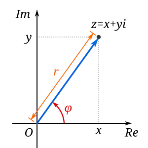
Complex numbers can be expressed in two forms: Cartesian coordinates (${\displaystyle x+iy}$) or polar coordinates ${\displaystyle re^{i\theta }}$, where ${\displaystyle r}$ is the distance from the origin or modulus and ${\displaystyle \theta }$ is the angle relative to the positive ${\displaystyle x}$ axis or argument.

For complex functions ${\displaystyle f(z)}$ of complex variables ${\displaystyle z}$ we can draw a 3-dimensional graph where the ${\displaystyle x}$ and ${\displaystyle y}$ axes are the real and imaginary components respectively of the ${\displaystyle z}$ variable and the ${\displaystyle z}$ axis is either the the modulus or the argument of the function ${\displaystyle f(z)}$.

For roots and logarithms, if we use the argument of the function for the ${\displaystyle z}$ axis, we see a discontinuity that restricts where we can draw the contour when we want to integrate the function.

The gap you can see along the negative ${\displaystyle x}$ axis is the discontinuity.

Root and logarithmic functions do not have poles about which we can do a Laurent expansion. Instead, we need to draw our contours to avoid these gaps or discontinuities. This is why in what follows we use contours with slits or wedges taken out of them.

Proof due to Sedgewick, Flajolet and Odlyzko^[3]

The proof for the estimate of the coefficient of the first term.

By Cauchy's coefficient formula

${\displaystyle [z^{n}](1-z)^{\alpha }\left({\frac {1}{z}}\log {\frac {1}{1-z}}\right)^{\gamma }\left({\frac {1}{z}}\log \left({\frac {1}{z}}\log {\frac {1}{1-z}}\right)\right)^{\delta }={\frac {1}{2\pi i}}\int _{C}(1-z)^{\alpha }\left({\frac {1}{z}}\log {\frac {1}{1-z}}\right)^{\gamma }\left({\frac {1}{z}}\log \left({\frac {1}{z}}\log {\frac {1}{1-z}}\right)\right)^{\delta }{\frac {dz}{z^{n+1}}}}$

where ${\displaystyle C}$ is a circle centred at the origin.

It is possible to deform ${\displaystyle C}$ without changing the value of the contour integral above.

We will deform ${\displaystyle C}$ by putting a slit through it along the real axis from 1 to ${\displaystyle +\infty }$.

We increase the radius of the circle to ${\displaystyle \infty }$, which reduces its contribution to the integrand to 0.

Therefore, the contour integration around ${\displaystyle C}$ above is equivalent to the contour integration around the contour which starts at ${\displaystyle Re(+\infty )}$, winds around 1 and ends at ${\displaystyle Re(+\infty )}$, which we will call ${\displaystyle {H_{\frac {1}{n}}}}$.

While we don't know much about the behaviour of the integral around the contour ${\displaystyle {H_{\frac {1}{n}}}}$, we do know about a similar contour ${\displaystyle H_{1}}$ (the Hankel contour) which winds around the origin at a distance of 1.

We can calculate the integral around ${\displaystyle {H_{\frac {1}{n}}}}$ by turning it into an integral around ${\displaystyle H_{1}}$. Formally:

${\displaystyle \int _{H_{\frac {1}{n}}}f(z)dz=\int _{\psi ^{-1}\circ H_{\frac {1}{n}}}f(\psi (\zeta ))\psi '(\zeta )d\zeta .}$^[4]

Such that ${\displaystyle \psi ^{-1}\circ H_{\frac {1}{n}}=H_{1}}$.

Informally this means we want to find a function ${\displaystyle \psi ^{-1}(t)}$ which turns the contour ${\displaystyle {H_{\frac {1}{n}}}}$ into ${\displaystyle H_{1}}$. Geometrically, we move the contour to the left by 1 and multiply it by ${\displaystyle n}$:

${\displaystyle \psi ^{-1}(t)=n(t-1)}$

But, we still want the integrand around ${\displaystyle H_{1}}$ to be equivalent to the integrand around ${\displaystyle {H_{\frac {1}{n}}}}$. We do this by dividing the variable by ${\displaystyle n}$ and adding 1:

${\displaystyle \psi (t)=1+{\frac {t}{n}}}$

Therefore, we get the following substitution^[5]:

${\displaystyle {\begin{aligned}{\frac {1}{2\pi i}}\int _{H_{\frac {1}{n}}}(1-z)^{\alpha }\left({\frac {1}{z}}\log {\frac {1}{1-z}}\right)^{\gamma }\left({\frac {1}{z}}\log \left({\frac {1}{z}}\log {\frac {1}{1-z}}\right)\right)^{\delta }{\frac {dz}{z^{n+1}}}&={\frac {1}{2\pi i}}\int _{\psi ^{-1}\circ H_{\frac {1}{n}}}(1-(1+{\frac {t}{n}}))^{\alpha }\left({\frac {1}{1+{\frac {t}{n}}}}\log {\frac {1}{1-(1+{\frac {t}{n}})}}\right)^{\gamma }\left({\frac {1}{1+{\frac {t}{n}}}}\log \left({\frac {1}{1+{\frac {t}{n}}}}\log {\frac {1}{1-(1+{\frac {t}{n}})}}\right)\right)^{\delta }{\frac {1}{n}}{\frac {dt}{(1+{\frac {t}{n}})^{n+1}}}\\&={\frac {n^{-a-1}}{2\pi i}}\int _{H_{1}}(-t)^{\alpha }\left(\log -{\frac {n}{t}}\right)^{\gamma }\left(\log \left({\frac {1}{1+{\frac {t}{n}}}}\log -{\frac {n}{t}}\right)\right)^{\delta }\left(1+{\frac {t}{n}}\right)^{-n-\gamma -\delta -1}dt\\&={\frac {n^{-a-1}}{2\pi i}}(\log n)^{\gamma }\int _{H_{1}}(-t)^{\alpha }\left(1-{\frac {\log(-t)}{\log n}}\right)^{\gamma }\left(\log \left({\frac {1}{1+{\frac {t}{n}}}}\log -{\frac {n}{t}}\right)\right)^{\delta }\left(1+{\frac {t}{n}}\right)^{-n-\gamma -\delta -1}dt\\&\sim {\frac {n^{-a-1}}{2\pi i}}(\log n)^{\gamma }\int _{H_{1}}(-t)^{\alpha }\left(\log \left({\frac {1}{1+{\frac {t}{n}}}}\log -{\frac {n}{t}}\right)\right)^{\delta }\left(1+{\frac {t}{n}}\right)^{-n-\gamma -\delta -1}dt\quad ({\text{as }}n\to \infty )\\&={\frac {n^{-a-1}}{2\pi i}}(\log n)^{\gamma }\int _{H_{1}}(-t)^{\alpha }\left(\log {\frac {1}{1+{\frac {t}{n}}}}+\log \log -{\frac {n}{t}}\right)^{\delta }\left(1+{\frac {t}{n}}\right)^{-n-\gamma -\delta -1}dt\\&\sim {\frac {n^{-a-1}}{2\pi i}}(\log n)^{\gamma }\int _{H_{1}}(-t)^{\alpha }\left(\log \log -{\frac {n}{t}}\right)^{\delta }\left(1+{\frac {t}{n}}\right)^{-n-\gamma -\delta -1}dt\quad ({\text{as }}n\to \infty )\\&={\frac {n^{-a-1}}{2\pi i}}(\log n)^{\gamma }(\log \log n)^{\delta }\int _{H_{1}}(-t)^{\alpha }\left(1-{\frac {\log \log(-t)}{\log \log n}}\right)^{\delta }\left(1+{\frac {t}{n}}\right)^{-n-\gamma -\delta -1}dt\\&\sim {\frac {n^{-a-1}}{2\pi i}}(\log n)^{\gamma }(\log \log n)^{\delta }\int _{H_{1}}(-t)^{\alpha }\left(1+{\frac {t}{n}}\right)^{-n-\gamma -\delta -1}dt\quad ({\text{as }}n\to \infty )\end{aligned}}}$

We have:

${\displaystyle \left(1+{\frac {t}{n}}\right)^{-n-\gamma -\delta -1}\sim e^{-t}}$ (as ${\displaystyle n\to \infty }$)

and:

${\displaystyle {\frac {1}{2\pi i}}\int _{H_{1}}(-t)^{\alpha }e^{-t}dt={\frac {1}{\Gamma (-\alpha )}}}$

Therefore,

${\displaystyle {\frac {1}{2\pi i}}\int _{H_{1}}(-t)^{\alpha }\left(1+{\frac {t}{n}}\right)^{-n-1}dt\sim {\frac {1}{2\pi i}}\int _{H_{1}}(-t)^{\alpha }e^{-t}dt={\frac {1}{\Gamma (-\alpha )}}}$^[6]

Putting it all together:

${\displaystyle {\begin{aligned}[z^{n}](1-z)^{\alpha }\left({\frac {1}{z}}\log {\frac {1}{1-z}}\right)^{\gamma }\left({\frac {1}{z}}\log \left({\frac {1}{z}}\log {\frac {1}{1-z}}\right)\right)^{\delta }&={\frac {1}{2\pi i}}\int _{C}(1-z)^{\alpha }\left({\frac {1}{z}}\log {\frac {1}{1-z}}\right)^{\gamma }\left({\frac {1}{z}}\log \left({\frac {1}{z}}\log {\frac {1}{1-z}}\right)\right)^{\delta }{\frac {dz}{z^{n+1}}}\\&={\frac {1}{2\pi i}}\int _{H_{\frac {1}{n}}}(1-z)^{\alpha }\left({\frac {1}{z}}\log {\frac {1}{1-z}}\right)^{\gamma }\left({\frac {1}{z}}\log \left({\frac {1}{z}}\log {\frac {1}{1-z}}\right)\right)^{\delta }{\frac {dz}{z^{n+1}}}\\&={\frac {n^{-a-1}}{2\pi i}}(\log n)^{\gamma }(\log \log n)^{\delta }\int _{H_{1}}(-t)^{\alpha }\left(1+{\frac {t}{n}}\right)^{-n-1}dt\\&\sim {\frac {n^{-a-1}}{2\pi i}}(\log n)^{\gamma }(\log \log n)^{\delta }\int _{H_{1}}(-t)^{\alpha }e^{-t}dt\\&={\frac {n^{-\alpha -1}}{\Gamma (-\alpha )}}(\log n)^{\gamma }(\log \log n)^{\delta }\end{aligned}}}$

Explanation and example from Flajolet and Sedgewick^[7].

In the below

${\displaystyle F(z)=(1-z)^{\alpha }\left({\frac {1}{z}}\log {\frac {1}{1-z}}\right)^{\gamma }\left({\frac {1}{z}}\log \left({\frac {1}{z}}\log {\frac {1}{1-z}}\right)\right)^{\delta }\quad (\alpha \notin \{0,1,2,\ldots \},\gamma ,\delta \notin \{1,2,\ldots \})}$

We will be making use of the "little o" notation.

${\displaystyle f(z)=o(g(z))}$ as ${\displaystyle z\to \zeta }$

which means

${\displaystyle \lim _{z\to \zeta }{\frac {f(z)}{g(z)}}=0}$

It also means for each ${\displaystyle \epsilon >0}$ there exists ${\displaystyle \delta >0}$ such that^[8]

${\displaystyle |z-\zeta |\leq \delta \implies f(z)\leq \epsilon g(z)}$

a fact we will use in the proof.

It is also useful to note

${\displaystyle f(z)=g(z)+o(g(z))\iff f(z)\sim g(z)}$

For the generating function ${\displaystyle f(z)}$:

1. Find ${\displaystyle f(z)}$'s singularity ${\displaystyle \zeta }$.
2. Construct the ${\displaystyle \Delta }$-domain at ${\displaystyle \zeta }$.
3. Check that ${\displaystyle f(z)}$ is analytic in the ${\displaystyle \Delta }$-domain.
4. Create an approximation of ${\displaystyle f(z)}$ near ${\displaystyle \zeta }$ of the form ${\displaystyle f(z)=F\left({\frac {z}{\zeta }}\right)+o\left(F\left({\frac {z}{\zeta }}\right)\right)}$.
5. The estimate of ${\displaystyle [(z/\zeta )^{n}]f(z)\sim {\frac {n^{-\alpha -1}}{\Gamma (-\alpha )}}(\log n)^{\gamma }(\log \log n)^{\delta }}$ or equivalently ${\displaystyle [z^{n}]f(z)\sim \zeta ^{-n}{\frac {n^{-\alpha -1}}{\Gamma (-\alpha )}}(\log n)^{\gamma }(\log \log n)^{\delta }}$.

As an example, we will use ${\displaystyle f(z)={\frac {e^{-z/2-z^{2}/4}}{\sqrt {1-z}}}}$. It has a branch point singularity at ${\displaystyle z=1}$.

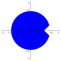
The ${\displaystyle \Delta }$-domain at 1 is a circle centred at the origin with radius ${\displaystyle R}$ with a triangle cut out of it with one vertex at 1 and edges of angles ${\displaystyle \phi }$ and ${\displaystyle -\phi }$. See image below. We use this domain as it allows us to make a proof later.

For ${\displaystyle f(z)}$ to be analytic in the ${\displaystyle \Delta }$-domain:

${\displaystyle f(z)=\sum _{n=0}^{\infty }a_{n}(z-z_{0})^{n}}$

for all ${\displaystyle z_{0}}$ in the ${\displaystyle \Delta }$-domain^[9].

Our example is analytic in the ${\displaystyle \Delta }$-domain because

• ${\displaystyle e^{-z/2-z^{2}/4}}$ is an entire function (i.e. has no singularities), which means it is analytic everywhere.
• ${\displaystyle {\frac {1}{\sqrt {1-z}}}}$ is analytic except for the slit along the real axis for ${\displaystyle z\geq 1}$.
• The product of two analytic functions is an analytic function on the same domain^[10]. Therefore, ${\displaystyle {\frac {e^{-z/2-z^{2}/4}}{\sqrt {1-z}}}}$ is analytic on the entire complex domain, including the ${\displaystyle \Delta }$-domain, except for the real axis ${\displaystyle z\geq 1}$.

We want an approximation of the form ${\displaystyle f(z)=F\left({\frac {z}{\zeta }}\right)+o\left(F\left({\frac {z}{\zeta }}\right)\right)\quad (z\to \zeta )}$ (where in our example we set ${\displaystyle \gamma ,\delta =0}$ and ${\displaystyle \zeta =1}$).

Normally, this will be in the form of a Taylor series expansion.

For our example, doing the Taylor Expansion near to 1:

${\displaystyle e^{-z/2-z^{2}/4}=e^{-3/4}+e^{-3/4}(1-z)+{\frac {e^{-3/4}}{4}}(1-z)^{2}+\cdots }$

${\displaystyle {\frac {1}{\sqrt {1-z}}}={\frac {1}{\sqrt {1-z}}}}$

${\displaystyle {\frac {e^{-z/2-z^{2}/4}}{\sqrt {1-z}}}={\frac {e^{-3/4}}{\sqrt {1-z}}}+e^{-3/4}{\sqrt {1-z}}+{\frac {e^{-3/4}}{4}}(1-z)^{\frac {3}{2}}+\cdots }$

Therefore:

${\displaystyle {\frac {e^{-z/2-z^{2}/4}}{\sqrt {1-z}}}={\frac {e^{-3/4}}{\sqrt {1-z}}}+o({\frac {e^{-3/4}}{\sqrt {1-z}}})}$

Then ${\displaystyle [z^{n}]f(z)\sim {\frac {n^{-\alpha -1}}{\Gamma (-\alpha )}}(\log n)^{\gamma }(\log \log n)^{\delta }}$.

Therefore, in our example:

${\displaystyle [z^{n}]{\frac {e^{-z/2-z^{2}/4}}{\sqrt {1-z}}}\sim {\frac {e^{-3/4}}{\sqrt {\pi n}}}}$

The proof of this comes from the fact that:

1. ${\displaystyle [z^{n}]f(z)=\zeta ^{-n}[(z/\zeta ^{n}]f(z)}$
2. ${\displaystyle [(z/\zeta )^{n}]f(z)=[(z/\zeta )^{n}]F(z/\zeta )+[(z/\zeta )^{n}]o(F(z/\zeta ))}$
3. the coefficients of the first term ${\displaystyle [(z/\zeta )^{n}]F(z/\zeta )\sim {\frac {n^{-\alpha -1}}{\Gamma (-\alpha )}}(\log n)^{\gamma }(\log \log n)^{\delta }}$, which we get from the standard function scale.
4. and the coefficients of the second term ${\displaystyle [(z/\zeta )^{n}]o(F(z/\zeta ))=o\left(n^{-\alpha -1}(\log n)^{\gamma }(\log \log n)^{\delta }\right)}$ which we do in #Proof of error term. This is also the reason why we need to use the ${\displaystyle \Delta }$-domain.

Proof from Flajolet and Odlyzko^[11], Flajolet and Sedgewick^[12] and Pemantle and Wilson^[13].

We get the estimate of the coefficient for the second term from Cauchy's coefficient formula:

${\displaystyle [z^{n}]o(F(z))={\frac {1}{2i\pi }}\int _{\gamma }o(F(z)){\frac {dz}{z^{n+1}}}}$

where ${\displaystyle \gamma }$ is any closed contour inside the ${\displaystyle \Delta }$-domain. See the red line in the image below.

We split ${\displaystyle \gamma }$ into four parts such that ${\displaystyle \gamma =\gamma _{1}\cup \gamma _{2}\cup \gamma _{3}\cup \gamma _{4}}$.

${\displaystyle \gamma _{1}=\{z\mid |z-1|={\frac {1}{n}},|arg(z-1)|\geq \phi \}}$

${\displaystyle \gamma _{2}=\{z\mid |z-1|\geq {\frac {1}{n}},|z|\leq r,|arg(z-1)|=\phi \}}$

${\displaystyle \gamma _{3}=\{z\mid |z|=r>1,|arg(z-1)|\geq \phi \}}$

${\displaystyle \gamma _{4}=\{z\mid |z-1|\geq {\frac {1}{n}},|z|\leq r,|arg(z-1)|=-\phi \}}$

${\displaystyle {\frac {1}{2i\pi }}\int _{\gamma }o(F(z)){\frac {dz}{z^{n+1}}}={\frac {1}{2i\pi }}\int _{\gamma _{1}}o(F(z)){\frac {dz}{z^{n+1}}}+{\frac {1}{2i\pi }}\int _{\gamma _{2}}o(F(z)){\frac {dz}{z^{n+1}}}+{\frac {1}{2i\pi }}\int _{\gamma _{3}}o(F(z)){\frac {dz}{z^{n+1}}}+{\frac {1}{2i\pi }}\int _{\gamma _{4}}o(F(z)){\frac {dz}{z^{n+1}}}}$

Contribution of ${\displaystyle \gamma _{1}}$:

The maximum of ${\displaystyle F(z)}$ on ${\displaystyle \gamma _{1}}$ is when ${\displaystyle z=1-{\frac {1}{n}}}$

${\displaystyle o(F(z))\leq \epsilon n^{-\alpha }(\log n)^{\gamma }(\log {\frac {1}{1-{\frac {1}{n}}}}+\log \log n)^{\delta }{\frac {1}{(1-{\frac {1}{n}})^{\gamma +\delta }}}\sim \epsilon n^{-\alpha }(\log n)^{\gamma }(\log \log n)^{\delta }\quad ({\text{as }}n\to \infty )}$

The maximum of ${\displaystyle {\frac {1}{z^{n+1}}}}$ on ${\displaystyle \gamma _{1}}$ is

${\displaystyle {\frac {1}{(1-{\frac {1}{n}})^{n+1}}}\leq 2e}$

The maximum of ${\displaystyle dz}$ on ${\displaystyle \gamma _{1}}$ is ${\displaystyle {\frac {2\pi }{n}}}$

${\displaystyle {\frac {1}{2i\pi }}\int _{\gamma _{1}}o(F(z)){\frac {dz}{z^{n+1}}}\leq \epsilon 2en^{-\alpha -1}(\log n)^{\gamma }(\log \log n)^{\delta }=o(n^{-\alpha -1}(\log n)^{\gamma }(\log \log n)^{\delta })}$

Contribution of ${\displaystyle \gamma _{2}}$ and ${\displaystyle \gamma _{4}}$:

We parameterise the contour ${\displaystyle \gamma _{2}}$ by converting ${\displaystyle z}$ to polar form by ${\displaystyle z=1+{\frac {t}{n}}e^{i\phi }}$, so that ${\displaystyle \gamma _{2}}$ is a function of ${\displaystyle t}$ from ${\displaystyle 1}$ to ${\displaystyle En}$. ${\displaystyle E}$ is the positive solution to the equation ${\displaystyle |1+Ee^{i\phi }|=r}$, so that the contour joins ${\displaystyle \gamma _{3}}$:

${\displaystyle \int _{\gamma _{2}}o(F(z)){\frac {dz}{z^{n+1}}}\leq \int _{1}^{En}|F(1+{\frac {t}{n}}e^{i\phi })|{\frac {e^{i\phi }dt}{n(1+{\frac {t}{n}}e^{i\phi })^{n+1}}}}$

But, remember that the little o relation only holds within a particular ${\displaystyle \delta }$ of ${\displaystyle 1}$. We know that ${\displaystyle {\frac {\log ^{2}n}{n}}}$ tends to zero as ${\displaystyle n}$ increases, and therefore, for any ${\displaystyle \epsilon }$, we choose an ${\displaystyle n}$ big enough so that ${\displaystyle {\frac {\log ^{2}n}{n}}\leq \delta }$. We split the integral above into two at ${\displaystyle \log ^{2}n}$, so that ${\displaystyle {\frac {t}{n}}e^{i\phi }\leq \delta }$:

${\displaystyle \int _{1}^{En}|F(1+{\frac {t}{n}}e^{i\phi })|{\frac {e^{i\phi }dt}{n(1+{\frac {t}{n}}e^{i\phi })^{n+1}}}=\int _{1}^{\log ^{2}n}\epsilon |F(1+{\frac {t}{n}}e^{i\phi })|{\frac {e^{i\phi }dt}{n(1+{\frac {t}{n}}e^{i\phi })^{n+1}}}+\int _{\log ^{2}n}^{En}F(1+{\frac {t}{n}}e^{i\phi }){\frac {e^{i\phi }dt}{n(1+{\frac {t}{n}}e^{i\phi })^{n+1}}}}$

The first term in the sum:

${\displaystyle {\begin{aligned}\int _{1}^{\log ^{2}n}\epsilon |F(1+{\frac {t}{n}}e^{i\phi })|{\frac {e^{i\phi }dt}{n(1+{\frac {t}{n}}e^{i\phi })^{n+1}}}&\leq {\frac {1}{2i\pi }}\int _{1}^{\infty }\epsilon |{\frac {t}{n}}e^{i\phi }|^{\alpha }|\log {\frac {n}{te^{i\phi }}}|^{\gamma }|\log({\frac {1}{1+{\frac {t}{n}}e^{i\phi }}}\log {\frac {n}{te^{i\phi }}})|^{\delta }|1+{\frac {t}{n}}e^{i\phi }|^{-n-\gamma -\delta -1}{\frac {e^{i\phi }dt}{n}}\\&\leq {\frac {1}{2i\pi }}\epsilon \left({\frac {e^{i\phi }}{n}}\right)^{\alpha +1}\left(\log {\frac {n}{e^{i\phi }}}\right)^{\gamma }\int _{1}^{\infty }|t|^{\alpha }|\log({\frac {1}{1+{\frac {t}{n}}e^{i\phi }}}\log {\frac {n}{e^{i\phi }}})|^{\delta }|1+{\frac {t}{n}}e^{i\phi }|^{-n-\gamma -\delta -1}dt\\&\sim {\frac {1}{2i\pi }}\epsilon \left({\frac {e^{i\phi }}{n}}\right)^{\alpha +1}\left(\log {\frac {n}{e^{i\phi }}}\right)^{\gamma }\left(\log \log {\frac {n}{e^{i\phi }}}\right)^{\delta }\int _{1}^{\infty }|t|^{\alpha }|1+{\frac {t}{n}}e^{i\phi }|^{-n-\gamma -\delta -1}dt\quad ({\text{as }}n\to \infty )\\\end{aligned}}}$

${\displaystyle |1+{\frac {e^{i\phi }t}{n}}|\geq 1+Re({\frac {e^{i\phi }t}{n}})=1+{\frac {t\cos \phi }{n}}}$^[14] (where ${\displaystyle Re(x)}$ is the real part of x).

${\displaystyle \int _{1}^{\log ^{2}n}|t|^{\alpha }|1+{\frac {t}{n}}e^{i\phi }|^{-n-\gamma -\delta -1}dt\leq \int _{1}^{\infty }|t|^{\alpha }|1+{\frac {t}{n}}e^{i\phi }|^{-n-\gamma -\delta -1}dt\leq \int _{1}^{\infty }|t|^{\alpha }\left(1+{\frac {t\cos \phi }{n}}\right)^{-n-\gamma -\delta -1}dt\leq \int _{1}^{\infty }t^{a}e^{-t\cos \phi }dt\quad ({\text{as }}n\to \infty )}$

This converges to a constant ${\displaystyle L}$. Therefore:

${\displaystyle {\frac {1}{2i\pi }}\epsilon \left({\frac {e^{i\phi }}{n}}\right)^{\alpha +1}\left(\log {\frac {n}{e^{i\phi }}}\right)^{\gamma }\left(\log \log {\frac {n}{e^{i\phi }}}\right)^{\delta }\int _{1}^{\infty }|t|^{\alpha }|1+{\frac {t}{n}}e^{i\phi }|^{-n-\gamma -\delta -1}dt={\frac {L}{2i\pi }}\epsilon \left({\frac {e^{i\phi }}{n}}\right)^{\alpha +1}\left(\log {\frac {n}{e^{i\phi }}}\right)^{\gamma }\left(\log \log {\frac {n}{e^{i\phi }}}\right)^{\delta }=o(n^{-\alpha -1}(\log n)^{\gamma }(\log \log n)^{\delta })\quad (n\to \infty )}$

The second term in the sum:

${\displaystyle {\begin{aligned}\int _{\log ^{2}n}^{En}F(1+{\frac {t}{n}}e^{i\phi }){\frac {e^{i\phi }dt}{n(1+{\frac {t}{n}}e^{i\phi })^{n+1}}}&\leq {\frac {1}{2i\pi }}\left({\frac {e^{i\phi }}{n}}\right)^{\alpha +1}\left(\log {\frac {n}{e^{i\phi }}}\right)^{\gamma }\left(\log \log {\frac {n}{e^{i\phi }}}\right)^{\delta }\int _{\log ^{2}n}^{En}|t|^{\alpha }\left(1+{\frac {\log ^{2}n\cos \phi }{n}}\right)^{-n-\gamma -\delta -1}dt\\&\leq {\frac {1}{2i\pi }}\left({\frac {e^{i\phi }}{n}}\right)^{\alpha +1}\left(\log {\frac {n}{e^{i\phi }}}\right)^{\gamma }\left(\log \log {\frac {n}{e^{i\phi }}}\right)^{\delta }\int _{\log ^{2}n}^{En}|t|^{\alpha }e^{-\log ^{2}n\cos \phi }dt\\&\leq {\frac {1}{2i\pi }}\left({\frac {e^{i\phi }}{n}}\right)^{\alpha +1}\left(\log {\frac {n}{e^{i\phi }}}\right)^{\gamma }\left(\log \log {\frac {n}{e^{i\phi }}}\right)^{\delta }{\frac {|En|^{\alpha }}{n^{\log n\cos \phi }}}En\end{aligned}}}$

${\displaystyle n^{\log n\cos \phi }}$ grows faster with ${\displaystyle n}$ than ${\displaystyle |En|^{\alpha +1}}$, so ${\displaystyle {\frac {|En|^{\alpha +1}}{n^{\log n\cos \phi }}}\to 0}$ as ${\displaystyle n\to \infty }$. Therefore:

${\displaystyle {\frac {1}{2i\pi }}\left({\frac {e^{i\phi }}{n}}\right)^{\alpha +1}\left(\log {\frac {n}{e^{i\phi }}}\right)^{\gamma }\left(\log \log {\frac {n}{e^{i\phi }}}\right)^{\delta }{\frac {|En|^{\alpha +1}}{n^{\log n\cos \phi }}}=o(n^{-\alpha -1}(\log n)^{\gamma }(\log \log n)^{\delta })\quad (n\to \infty )}$

A similar argument applies to ${\displaystyle \gamma _{4}}$.

Contribution of ${\displaystyle \gamma _{3}}$:

By Cauchy's inequality

${\displaystyle {\frac {1}{2i\pi }}\int _{\gamma _{3}}o(F(z)){\frac {dz}{z^{n+1}}}\leq {\frac {\max _{|z|=r}F(z)}{r^{n}}}}$

meaning the contribution of the integral around ${\displaystyle \gamma _{3}}$ is exponentially small as ${\displaystyle n\to \infty }$ and can be discarded.

The above assumes only one singularity ${\displaystyle \zeta }$. But, it can be generalised for functions with multiple singularities.

In the case of multiple singularities, the separate contributions from each of the singularities, as given by the basic singularity analysis process, are to be added up.

—Flajolet and Sedgewick 2009, pp. 398.

Theorem from Flajolet and Sedgewick^[15].

Assume ${\displaystyle f(z)}$ is analytic on the disc ${\displaystyle |z|<\rho }$, has a finite number of singularities on the circle ${\displaystyle |z|=\rho }$ and ${\displaystyle f(z)}$ is analytic on the ${\displaystyle \Delta }$-domain with multiple indents, one at each singularity.

If for each singularity ${\displaystyle \zeta _{i}}$ (for ${\displaystyle i=1,2,\cdots ,r}$):

${\displaystyle f(z)\sim \left(1-{\frac {z}{\zeta _{i}}}\right)^{\alpha _{i}}\left({\frac {1}{\frac {z}{\zeta _{i}}}}\log {\frac {1}{1-{\frac {z}{\zeta _{i}}}}}\right)^{\gamma _{i}}\left({\frac {1}{\frac {z}{\zeta _{i}}}}\log \left({\frac {1}{\frac {z}{\zeta _{i}}}}\log {\frac {1}{1-{\frac {z}{\zeta _{i}}}}}\right)\right)^{\delta _{i}}\quad ({\text{as }}z\to \zeta _{i})}$

then:

${\displaystyle [z^{n}]f(z)\sim \sum _{i=0}^{r}\zeta _{i}^{n}{\frac {n^{-{\alpha _{i}}-1}}{\Gamma (-{\alpha _{i}})}}(\log n)^{\gamma _{i}}(\log \log n)^{\delta _{i}}\quad ({\text{as }}n\to \infty )}$

• Flajolet, Philippe; Odlyzko, Andrew (1990). "Singularity analysis of generating functions" (PDF). SIAM Journal on Discrete Mathematics. 1990 (3).
• Flajolet, Philippe; Sedgewick, Robert (2009). Analytic Combinatorics (PDF). Cambridge University Press.
• Lang, Serge (1999). Complex Analysis (4th ed.). Springer Science+Business Media, LLC.
• Lorenz, Dirk (2011). "Substitution and integration by parts for functions of a complex variable". Retrieved 27 November 2022.
• Pemantle, Robin; Wilson, Mark C. (2013). Analytic Combinatorics in Several Variables (PDF). Cambridge University Press.
• Sedgewick, Robert. "6. Singularity Analysis" (PDF). Retrieved 13 November 2022.
• Stroud, K. A. (2003). Advanced Engineering Mathematics (4th ed.). Palgrave Macmillan.