OpenSCAD User Manual/Importing Geometry
Importing 3D Solids
In older versions of the application files of each format were imported using a module specific to it. These older modules are deprecated in newer versions but are still documented in this page.
Currently the import() Object Module processes each type of file according to its file extension to instantiate imported objects. [Note: Requires version 2015.03]
There are some other, purpose specific, import methods in the app:
- A '.csg' geometry file
- may be imported by an
include <filename.csg>statement. - A '.png' image
- The import image option of the surface() object module may be used to apply a height map to a surface.
- data in a text file
- The import numeric data of the surface() object module may also be used to apply a height map.
- data in a JSON file
- The import() function may can read structured data into an object that can then be processed by a script.
Include <"filename.csg">
A .csg format file is a type of geometry file exported from OpenSCAD using a subset of its programming language.
As such the shapes described by it may be imported into a program using the include <filename.csg> statement.
Import() Object Module
This is an Object Module that imports geometry for use in the script. The extension on the filename informs the module as to which input processor to use.
The import() function is a separate component for bringing in structured data from a JSON file.
Parameters
- file
- A string containing a filename and extension of form "filename.ext". The location of the file is the same as the script's file. Refer to the File System Issues page for other file path options and platform specific information.
filename- deprecated - a filename of form "filename.ext". Use "file" parameter.
- origin
- vector of form [xcoord,ycoord]
- scale
- number. A scale factor to apply to the model
- width
- number
- height
- number
- dpi
- non-negative integer >= 0.001. The Dots Per Inch value is used importing a SVG or DXF file to correctly size the generated geometry.
- center
- Boolean. When true the object is centered in the X-Y plane at the origin. [Note: Requires version Development snapshot]
- convexity
- non-negative integer. The convexity parameter specifies the maximum number of front sides (or back sides) a ray intersecting the object might penetrate. This parameter is needed only for correctly displaying the object in OpenCSG preview mode and has no effect on the polyhedron rendering. Optional.
- id
- String. For SVG import only, the id of an element or group to import. Optional. [Note: Requires version Development snapshot]
- layer
- For DXF and SVG import only, specify a specific layer to import. Optional.
layername- [Deprecated: layername will be removed in a future release. Use layer instead]
- $fn
- Number, default 0. The number of polygon segments to use when converting circles, arcs, and curves to polygons. [Note: Requires version Development snapshot]
- $fa
- Number, default 12. The minimum angle step to use when converting circles and arcs to polygons. [Note: Requires version Development snapshot]
- $fs
- Number, default 2. The minimum segment length to use when converting circles and arcs to polygons. [Note: Requires version Development snapshot]
3D Geometry Formats
There is a concise comparison of the commonly used file formats in 3D printing on the AnyCubic website that may be of interest.
These are the file formats recognized by import():
- OBJ
- OBJect data file by Wavefront
- AMF
- Additive Manufacturing Files include color, texture, and other meta data in addition to a 3D polygonal geometry but is deprecated as it has not achieved much acceptance in the industry.
- 3MF
- 3D Manufacturing Format XML data file
- CSG
- solid geometry format of OpenSCAD programming language
- STL
- STereoLithography file format by 3D Systems for describing polygons in a 3D coordinate space. Replaced by Additive Manufacturing Format (.amf)
- OFF
- Object File Format
- NEF3
- a CGAL geometry data format from a Nef Polygon object (ref section 15.6). It is used mostly by the OpenSCAD dev group as a debugging tool when building test cases for upstream reporting to CGAL.
2D Geometry Formats
Shapes drawn in two dimensional formats may also be imported by the import() module, as documented in the Import 2D page.
Image Formats
- PNG
- Portable Network Graphics image file. As already mentioned, the surface() method is able to derive a gray scale value from each pixel to apply to a surface as a height map.
import() Function - JSON only
[Note: Requires version Development snapshot]
This function returns an object with the structured data from a valid JSON file. Although it has the same name as the import() Module it is functionally separate in that it may only be used in an assignment statement and may not be the target action of an Operator Module.
/* "people.json" contains:
{"people":[{"name":"Helen", "age":19}, {"name":"Chris", "age":32}]}
*/
pf=import( file = "people.json" );
echo(pf);
people = pf.people;
for( p=people) {
	echo(str( p.name, ": ", p.age));
    }
or even
 people = import( file = "people.json" ).people;
 for( p=people) {
	 echo(str( p.name, ": ", p.age));
     }
both of which give the data about Helen and Chris:
ECHO: { people = [{ age = 19; name = "Helen"; }, { age = 32; name = "Chris"; }]; }
ECHO: "Helen: 19"
ECHO: "Chris: 32"
Surface() Object Module: Apply a Height Map
The Surface module draws a surface based on the Height map information given either as numbers in a text data file, or by interpreting the luminance of each pixel in a PNG image file (only).
The generated surface is normally drawn from the (0,0) origin in the +X,+Y quadrant. The extent of the drawn surface is either:
- data file - the number of columns and rows in the file
- image - the number of pixels in each direction of the image.
To make a surface of size (m,n) there must be n rows of numbers, with m values on each row.
Height values from an image file are massaged to the range of 0-100 and so will not have negative values, unless the invert option changes the sign of all the height values.
Height values are applied starting at the [0,0] corner. The column index and the X coordinate are both increased by one and the next value applied at the next position on the surface. Continue like this to the end of the row and then increase the Y coordinate, and the row index, by one as the row is completed. Repeat until all the rows are processed.
For a data file of size (m,n) the generated surface is grid of squares with the height value applied at the left-lower corner (as seen here). The n-th row of heights will be on the top vertices of the squares along the top edge of the surface:
 ^  [x,y+n] [x+m,y+n]
 |
 y  [x,y]   [x+m,y]
[0,0] x-->
A one unit thick base is drawn downwards under the generated surface from the level of the smallest value in the data file, including when heights have negative values. This means that when least height value is zero the base will extend down to z=-1.
Parameters
- filename
- Required String. The filename may include an absolute or a relative path to the height map data file. There is no default so the .png extension must be explicitly given.
- center
- Optional Boolean, default=
falseto draw in the +X,+Y quadrant. Whentruethe surface is centered on the X-Y origin. - invert
- Optional Boolean, default=false. Limitation: Only applies to image based maps
. Inverts how the pixel values are interpreted into height values.[Note: Requires version 2015.03]
- convexity
- Integer, default=1. Higher values improve preview rendering of complex shapes. Limitation: Only used by OpenCSG Preview
Text Data Format
A text data height map is simply rows of whitespace separated, floating point numbers. The values may be written as integers, floating point with decimal fractions, or using exponential notation such as 1.25e2 for 125.
Hex values are not accepted but may not give a warning.
Consider a data file with n rows and m values on each, thus having size (m,n). The X position of each data point is given by their position along their row, and the Y by the row. The implicit indexing starts at the beginning of the file with the first row being at Y=0 and the first point on each row at X=0. The X and Y positions increment by one until X=m and Y=n, which means that the last row of values is the farthest edge of the generated surface.
The appearance of a hash sign ('#') as the first, non-whitespace character on a line marks it as a comment. A hash mark following numbers on a row cause a lexical fault making the data file unreadable.
Examples Using Data Map
//surface.scad
surface(file = "surface.dat", center = true, convexity = 5);
%translate([0,0,5]) cube([10,10,10], center = true);
The transparent cube shows the extent of the data space, and that the base extends downwards to Y=-1.
#surface.dat
10 9 8 7 6 5 5 5 5 5
 9 8 7 6 6 4 3 2 1 0
 8 7 6 6 4 3 2 1 0 0
 7 6 6 4 3 2 1 0 0 0
 6 6 4 3 2 1 1 0 0 0
 6 6 3 2 1 1 1 0 0 0
 6 6 2 1 1 1 1 0 0 0
 6 6 1 0 0 0 0 0 0 0
 3 1 0 0 0 0 0 0 0 0
 3 0 0 0 0 0 0 0 0 0
Result:

One may use an application like Octave or Matlab to make a data file. This is a small Matlab script that superimposes two sine waves to create a 3D surface:
d = (sin(1:0.2:10)' * cos(1:0.2:10)) * 10;
save("-ascii", "example010.dat", "d");
The data file can then be used to draw the surface three ways:
//draw an instance of the surface
surface(file = "example010.dat", center = true);
//draw another instance, now rotated
translate(v = [70, 0, 0])
  rotate(45, [0, 0, 1])
    surface(file = "example010.dat", center = true);
// and two last instances, intersected
translate(v = [35, 60, 0])
intersection() {
  surface(file = "example010.dat", center = true);
    rotate(45, [0, 0, 1])
      surface(file = "example010.dat", center = true);
}

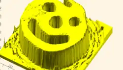
Image Base Height Maps
[Note: Requires version 2015.03]
Heights are calculated using the linear luminance for the sRGB color space (Y = 0.2126R + 0.7152G + 0.0722B) at each pixel to derive a Grayscale value, which are further scaled to the range [0:100]. For an image with a color space between black (rgb=0,0,0) and white (rgb=1,1,1) the gray scale will be the full range.
For an image with a a narrower range of colors the gray scale is likewise reduced, and the minimum and maximum luminance in the color range set the lowest and highest limits, respectively, on the surface's heights.
Note also that no base is added below the surface as is done for a data file surface. Squares at Z=0, black, do have a surface filled in so the entire area of the surface is continuous.
Normally, with invert=false, the surface will be drawn upwards from the X-Y plane with black being z=0 increasing up to white=100. When invert=true the shape is still drawn starting at the X-Y plane, but now downwards to white=-100.
Currently only PNG (.png) images are supported and only the RGB channels are used. Specifically, the alpha channel is ignored.
Example Using Invert
// Example 3a - apply a scale to the surface
scale([1, 1, 0.1])
  surface(file = "smiley.png", center = true);
scale([1, 1, 0.1])
  surface(file = "smiley.png", center = true, invert = true);
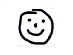
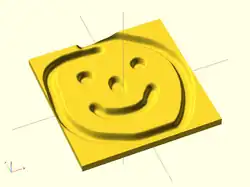
.png)

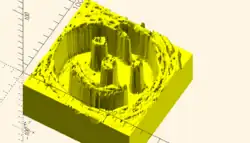
Note that the surfaces are above or, for the inverted surface, below, the X-Y plane, unlike Example 3
Example Grayscale Effects [Note: Requires version 2015.03]
surface(file = "BRGY-Grey.png", center = true, invert = false);
-
 PNG Test File
 -
 3D Surface