How do I calculate average of last 10 values from a row containing blanks

Question

I am trying to calculate golf handicaps for a league. There are 30 weeks on the schedule, and only the most recent 10 scores are used to calculate the handicap. The data looks like this:

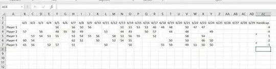
I am using this formula to calculate handicaps: =ROUND((AVERAGE(Q3:AD3)-54)*0.8,0)

Currently I have to adjust the range for each player, each week to include only their last 10 scores. How can I improve this formula to do that for me?

Answer 1

You need a more complex formula to consider last 10 cells with number:

=ROUND((AVERAGE(OFFSET(B2,0,LARGE(IF(B2:W2>0,COLUMN(B2:W2),""),10)-COLUMN(B2),1,COLUMN(W2)+1-LARGE(IF(B2:W2>0,COLUMN(B2:W2),""),10)))-54)*0.8,0)

where:

• LARGE(IF(B2:W2>0,COLUMN(B2:W2),""),10) gets the column number of the first number from the 10
• OFFSET(B2,0,LARGE(...)-COLUMN(B2),1,COLUMN(W2)+1-LARGE(...),10))) creates a reference to the range containing the 10 numbers
• =ROUND((AVERAGE(OFFSET(...)-54)*0.8,0) is the calculation according to your original formula

This is an array formula, so after inserting you need to press Ctrl+Shift+Enter

The formula will be automatically updated if you insert / delete columns to / from after first column referenced and before last column referenced.