How to average the last N row in Excel 2019 with blank cells

Question

I'm trying to average the last N rows in Excel, but I have some blank (and merged) cells; in something like this:

Example

A
1
2
x
3
4
5
6
7
y
8
9
10

for example, wanting average the last four rows it should average A8 to A12 ignoring A9, which isn't a number.

Moreover, new rows will be added, so the average needs to be dinamic, always taking the last N compiled rows with numbers.

I found some article like this on the topic, but they all assume consecutive data, without addressing the case of some blank/text cell amid the data; this answer seems to tackle the issue, but I wasn't able to make those formulas work for me (and I'm not sure how to use that in the accepted answer, since it uses more than one column, while I only have one).

This and this too seems relevant too, but again I wasn't able to make them work in my case.

Is there a way to do this?

Answer 1

Here is one way you could try, in Excel 2019:

=AVERAGE(
         INDEX(A:A,
         AGGREGATE(14,7,ROW(A:A)/((ISNUMBER(A:A))*(A:A<>"")),4)):
         INDEX(A:A,
         MATCH(2,1/((ISNUMBER(A:A))*(A:A<>""))))
 )

---

Explanation:

• The following finds the cell position of the last numeric value

---

=MATCH(2,1/((ISNUMBER(A:A))*(A:A<>"")))

---

• Now, wrapping within INDEX() gives us the cell value of the specified row number.
• The following returns the 4th largest row number which has a value

---

=AGGREGATE(14,7,ROW(A:A)/((ISNUMBER(A:A))*(A:A<>"")),4)

---

• Similarly, wrapping within INDEX() shall produce the cell value of that specific row.
• The use of full lookup then the colon, then another full lookup gives Excel the hint it needs that it must return a reference.
• Therefore it makes a range of the two cells located and passes that to the AVERAGE() Function wrapping around everything else to return the desired output.
• Also, note based one's Excel Version, one may need to hit CTRL+SHIFT+ENTER while exiting the edit mode.

---

Perhaps with MS365:

=AVERAGE(TAKE(FILTER(A:A,(ISNUMBER(A:A)*(A:A<>"")),""),-4))

---

Answer 2

=AVERAGE(
    INDEX(
        $A:$A,
        LARGE(
            ISNUMBER($A$1:INDEX($A:$A, LOOKUP(2, 1 / $A:$A, ROW($A:$A)))) *
                ROW($A$1:INDEX($A:$A, LOOKUP(2, 1 / $A:$A, ROW($A:$A)))),
            {1; 2; 3; 4}
        )
    )
)

• LOOKUP(2,1/A:A,ROW(A:A)) returns the row number of the last cell that contains a number (errors are ignored by this function).
• We then use INDEX to create an array of the values
• Test them to see which are numbers
• Return the Row numbers for only the values which are numbers
• Use LARGE with an array argument to return the highest four row numbers {1;2;3;4}
• Use those Row numbers within the outer INDEX function to return the values contained in those Rows
• AVERAGE those four numbers.

Of course, with 365 you could use the much shorter:

=AVERAGE(TAKE(FILTER(A:A,ISNUMBER(A:A)),-4))

Answer 3

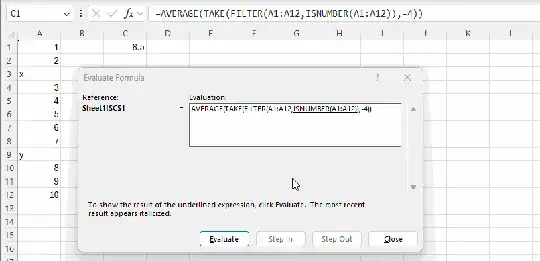
You can use this formula in Excel 365 to achieve your goal:
=AVERAGE(TAKE(FILTER(A1:A12,ISNUMBER(A1:A12)),-4))

• FILTER(A1:A12,ISNUMBER(A1:A12)) - removes non-numeric values
• TAKE(FILTER(...),-4)) - keeps the last four numbers
• =AVERAGE(...) - calculates average

Answer 4

Another option: =AVERAGE(INDEX(A:A,MATCH(2,1/A:A)-{3,2,1,0}))

Or in M365: =AVERAGE(TAKE(A:.A,-4))

(Average ignores non numeric values)