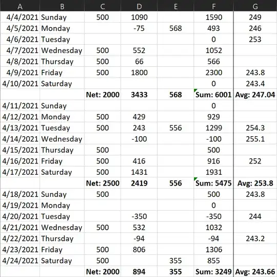
I am trying to find a way to get the average for the last 10 numerical values in column G. I am struggling a bit here as there are sporadic blanks in the column (not every row has a number in column G) and there are non-numerical values containing sub-averages combined with text in the column as well. Any help here would be appreciated. Here is some sample data:
Asked
Active
Viewed 259 times
2 Answers
1
If you have Office 365, you can use:
=LET(x,FILTER(G:G,ISNUMBER(G:G)),y,ROWS(x),AVERAGE(INDEX(x,SEQUENCE(10,,y-9,1))))
With earlier versions, try:
=AVERAGE(INDEX(G:G,AGGREGATE(14,6,1/ISNUMBER(G:G)*ROW(G:G),ROW(INDEX($A:$A,1):INDEX($A:$A,10)))))
This latter is an array formula. Depending on your version of Excel, you may need to enter/confirm it as an array formula by holding down ctrl + shift while hitting enter. If you do this correctly, Excel will place braces {...} around the formula seen in the formula bar.
Ron Rosenfeld
- 9,461
1
=AVERAGE(INDEX(G:G,LARGE(IF(ISNUMBER(G:G),ROW(G:G)),10)):G22)
G22 is a kludge. It is last entry in Table. You should be able to figure out how to get index.
Ron Rosenfeld
- 9,461
